SNP/Variant Calling Tutorial
From raw sequencing data to variant calling and annotation
Go to ai.tinybio.cloud/chat to chat with a life sciences focused ChatGPT.
This step-by-step tutorial will walk you through variant calling and variant annotation. You'll learn how to fetch whole-genome sequencing data, perform quality control and read mapping, and call small variants (i.e. SNPs and indels), before finally visualizing and annotating the obtained variants.
We’ll provide everything you need to follow along, including detailed instructions, scripts, estimated run times, and a guide to interpreting the results. All that's required is some very basic knowledge of Linux/Unix-like operating system commands and a regular laptop. Let's get started!
Creating a Computing Environment For SNP Calling
To perform variant calling and annotation, we’ll need to run several interlinking bioinformatics software packages. Installing these programs manually can be tedious and technically challenging due to their many dependencies. Our solution for this problem is Conda – a package manager that effortlessly handles software installations and compatibility. For more details about Conda please visit our dedicated guide. If you don’t have Conda yet, you can download it here.
After downloading and installing Conda (in our case, Miniconda, which is a minimal Conda installer), you can create and manage environments with all necessary software. For this guide, let's first create and activate an empty environment called varcall. In your terminal, run:
conda create -n varcall
conda activate varcall
Before installing software in the environment, however, we need to first configure Conda's so-called "channels" (via which software is downloaded). To do this, run the following commands:
conda config --add channels defaults
conda config --add channels bioconda
conda config --add channels conda-forge
conda config --set channel_priority strict
Now we can safely install our software. We'll perform these installations on-the-go in the following sections.
Variant Calling: A Quick Overview
In this tutorial, we will analyze the whole-genome sequencing data of a human fungal pathogen called Candida glabrata. As one of the major opportunistic yeast pathogens, this haploid yeast can quickly develop resistance to antifungal drugs.
We will be working with publicly available data from a study by Ksiezopolska et al (2021). For that study, researchers performed a large-scale, in-vitro evolution experiment by exposing C. glabrata to the main classes of antifungal drugs, including azoles and echinocandins. By performing DNA sequencing and variant calling of drug-exposed and non-exposed C. glabrata, the authors identified the genomic variants that turned this yeast into a drug-resistant pathogen.
For simplicity, we will only perform variant calling on one sample from this study, which was grown in the presence of the major antifungal drug fluconazole. The analyzed sample was subsequently sequenced using an Illumina HiSeq 2500 device, generating ~18 million paired-end reads with 125 bp read length. Given the size of the C. glabrata genome (~12MB), this yields a very high coverage of ~350 reads per position.
Variant Calling Data Pipeline
For this tutorial, we’ll fetch, clean, and analyze our data in a series of stages. Here is a simplified schematic showing the data analysis workflow we’ll follow:
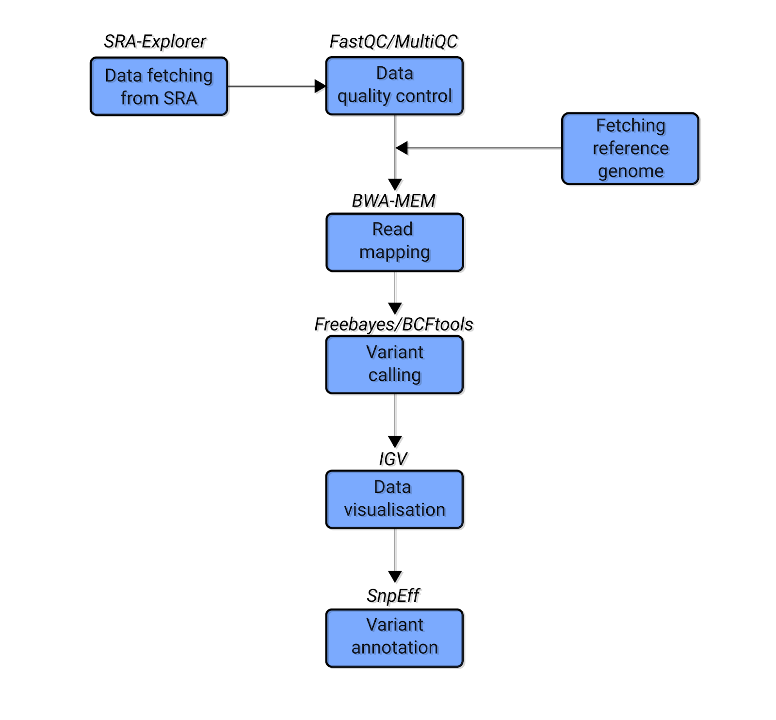
Fig. 1: The simplified schematic bioinformatics pipeline of the variant calling analysis covered in this tutorial. Blue boxes indicate the types of analysis. The text above the boxes indicates the software used for each analysis.
Let’s briefly explore the stages in this pipeline. First, we will use SRA Explorer to find and download the raw sequencing data. Then we will run a quality control analysis to ensure our data is high-quality. We will perform this step using FastQC and MultiQC (Ewels et al. 2016) software. In this case, our data is already high-quality (i.e. no low-quality bases or adapter sequences), meaning we can proceed to the next step without performing data trimming.
We will then map our reads against a corresponding reference genome for C. glabrata using bwa-mem (Li and Durbin, 2009). Next, we’ll perform variant calling using two popular pieces of software – bcftools (Li, 2011) and freebayes (Garrison and Marth, 2012). After obtaining variants, we will visualize them with Integrative Genomics Viewer (IGV) (Robinson et al. 2011). Finally, we will use SnpEff (Cingolani et al. 2012) software to systematically characterize different properties of the obtained data, thus making variant annotations.
Variant Calling: Detailed Data Prep Instructions
In this section, we will guide you through every step of the variant calling bioinformatics pipeline. We’ll provide detailed instructions, approximate run times, code samples, and scripts for each analysis.
To get started, activate the varcall Conda environment (if you haven’t done so already) by opening a terminal and running the following command:
conda activate varcall
Ready to proceed? Let's get started!
Hardware Requirements
We developed this tutorial on two separate machines. We'll give approximate runtimes for both of them so you can better estimate how long each step might take you:
- Workstation – a workstation with Intel Core i7-8700K CPU, 3.70GHz and 64 GB of RAM running on Open-Suse Leap 15.3
- Mac – a 2017 MacBook Pro 2.3 GHz Dual-Core Intel Core i5 with 8 GB of RAM, running on MacOS Monterey 12.4
Because we are analyzing data originating from a yeast whose reference genome is only 12 MB, all analyses require less than 8 GB of RAM. This means that the entire workflow can be easily performed on any modern desktop/laptop computer. You will only need around 5 GB of free hard drive space.
File System
To keep our analysis clean and tidy, we recommend creating these three folders in any convenient directory:
- raw_data
- ref_gen
- mapping
To create these directories, just run this command:
mkdir -p ./ref_gen/ ./mapping ./raw_data
These three folders (and various subdirectories which we'll create as we go) will contain our entire variant calling data analysis.
Fetching the Raw Variant Calling Datasets
Runtime: Depends on your internet connection speed. For 50Mbps, this step takes ~1 minute
In this section, we will fetch the raw sequencing data to be analyzed. To begin, go to SRA Explorer and enter the accession number SRR15498471. This will summon the whole genome sequencing data for a sample of C. glabrata grown in the presence of fluconazole. (This data originates from Ksiezopolska et al, 2021.)
Select the sample and add it to the collection. Then go to saved datasets and download the “Bash script for downloading FastQ files”. Now locate the downloaded file sra_explorer_fastq_download.sh in the raw_data folder and go to that folder:
cd raw_data/By default, SRA Explorer commands will rename downloaded files. In our case, this is not necessary. To prevent renaming, run this command:
sed "s/_WGS_of_Candida_glabrata_sample_CBS138_9H_FLZ//g" sra_explorer_fastq_download.sh > renamed_sra_explorer.shThe sed command above will simply remove the text “_WGS_of_Candida_glabrata_sample_CBS138_9H_FLZ” from the filenames we will download. After renaming, run this command to download the sequencing data:
bash renamed_sra_explorer.shWhen the downloading is finished, we will have two compressed fastq files (SRR15498471_1.fastq.gz and SRR15498471_2.fastq.gz) with forward and reverse reads, respectively.
Quality Control For Variant Calling Experiments
Runtime: 1 minute on the Workstation, 12 minutes on the Mac
In this section, we will perform quality control on our raw sequencing data. We will use FastQC to analyze the fastq files (i.e., our raw sequencing data) and MultiQC to aggregate the results of FastQC. Let’s begin by installing these programs in the Conda environment. In the activated varcall environment in your terminal, run this command:
conda install fastqc multiqc --channel conda-forge --channel bioconda --strict-channel-priorityNow that we've installed FastQC and MultiQC, let’s create a directory called fastqc and begin our FastQC analysis. Run these commands:
mkdir ./fastqc_initial
fastqc *fastq.gz -o ./fastqc -t 2
In this command, *fastq.gz instructs FastQC to analyze all files in the current directory ending with “fastq.gz” and store the results in the fastqc directory. (In our case, this is only two files – one for forward reads and one for reverse reads.) The option -t 2 tells FastQC to use two cores of the computer. If more cores are available, you can increase this value to speed up the analysis.
Now let’s check our quality control results. Since we only have two FastQC files to review, we could easily open and inspect them individually. But instead, let's aggregate them into a single report using MultiQC software. (This option is very valuable when there are many FastQC files and reviewing them individually would be tedious.)
First, navigate to the fastqc folder and run MultiQC:
cd ./fastqc
multiqc .
MultiQC will now scan the current directory and collect the output files of FastQC, generating a beautiful, aggregated html report. To inspect it, open the file multiqc_report.html in your web browser.
Let’s explore the main results of this report. First, you’ll notice a General Statistics plot (Fig. 2) which shows the overview of the data and its main parameters:
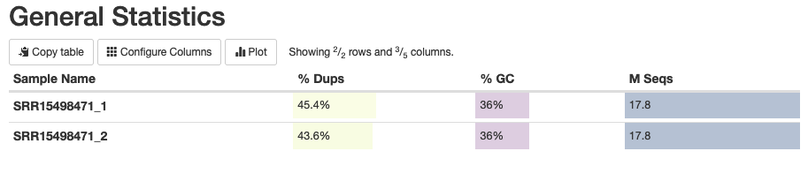
Fig. 2: The general statistics of the analyzed fastq samples, showing the sample names, duplication percentages, GC content percentages, and the number of sequencing reads.
Because we’re working with high-coverage data, the observed high rate (44-45%) of duplicated reads isn't surprising. (Note that some part of these duplicated reads may be PCR duplicates.) The GC content of 36% is also expected for C. glabrata, hinting that there is no contamination in our data. The final column of this indicates the number of sequenced reads, which in our case is 17.8 million for each direction.
Now let’s review the mean Phred quality scores for our read data. Phred score is one of the main quality indicators of NGS data, showing the reliability of each sequenced base. Your Phred score plot should look like this:
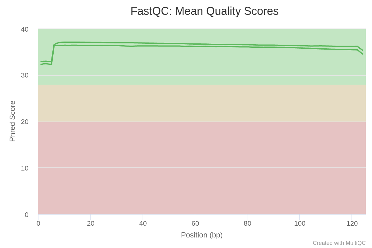
Fig. 3: Mean Phred-quality scores of each sample.
Phred score values between 30 and 40 are considered good scores. As you can see, the Phred quality of our data is very high, hovering around 35. (Learn more about Phred scores.)
Next, let’s check our read data for the presence of adapter sequences, which might have been introduced during the process of sample preparation. You should see a plot called “Adapter Content”, which shows that adapter sequences are practically absent from our data:
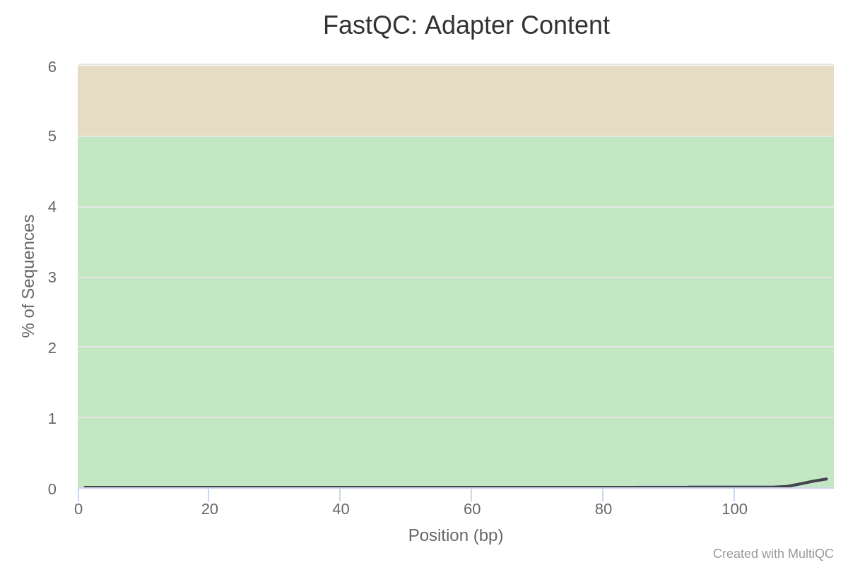
Fig. 4: Adapter content of the sequencing data.
As you can see, the general quality parameters of our data are all very high, meaning that it can be used immediately for downstream analysis. If the quality were low, it would be necessary to perform a trimming operation. To learn more about data trimming, check out our tutorials on RNA-Seq and ATAC-Seq analyses, both of which contain a data trimming step. In this case, we can skip the trimming step and proceed directly to genome indexing.
Genome Indexing & Read Mapping For Variant Calling Experiments
To perform variant calling, we first need to map our sequencing reads to the corresponding reference genome of C. glabrata. This step consists of two major parts – indexing the reference genome and read mapping itself (along with some auxiliary analyses). Let’s begin by downloading several pieces of software we’ll need.
For read mapping, we will use the popular software bwa with mem algorithm. We will also need Samtools (a powerful program for efficiently manipulating read alignment sam/bam files).
Install these programs in your varcall environment using this command:.
conda install bwa samtools --channel conda-forge --channel bioconda --strict-channel-priorityNow that our software is prepared, we can proceed with the analysis.
Genome Indexing
Runtime: ~10 seconds on both machines
In order to map our C. glabrata sequencing data to a reference genome, we first need to obtain and index a reference genome. To do so, run these commands:
cd ref_gen/
wget http://www.candidagenome.org/download/sequence/C_glabrata_CBS138/current/C_glabrata_CBS138_current_chromosomes.fasta.gz

wget http://www.candidagenome.org/download/gff/C_glabrata_CBS138/C_glabrata_CBS138_current_features.gff

gunzip C_glabrata_CBS138_current_chromosomes.fasta.gz
These commands take you to the ref_gen directory and download the reference genome and genome annotations of C. glabrata from the Candida Genome Database (Skrzypek et al. 2017). The gunzip command uncompresses the genome file.
To index the genome of C. glabrata, we will use a bash script called indexing.sh, which contains the following code:
bwa index -p cglab C_glabrata_CBS138_current_chromosomes.fastaThis code tells bwa to index the file C_glabrata_CBS138_current_chromosomes.fasta and create index files starting with “cglab”.
Run the script with this command:
bash indexing.sh Now that we’ve indexed our reference genome, our read data can be mapped to it.
Read Mapping
Runtime: 13 minutes on the Workstation, 22 minutes on the Mac
To begin mapping our sequencing reads to the reference genome of C. glabrata, first change your directory to mapping:
cd ../mapping/
The read mapping and subsequent auxiliary analyses will be done with the following script, called map_sort_index.sh:
bwa mem -t 2 ../ref_gen/cglab ../raw_data/SRR15498471_1.fastq.gz ../raw_data/SRR15498471_2.fastq.gz | samtools sort -@2 -o SRR15498471_sorted.bam -
samtools index SRR15498471_sorted.bam
samtools flagstat SRR15498471_sorted.bam > SRR15498471_mapping_stats.txt
Let’s explore how this script works:
bwa mem runs bwa software with the mem algorithm to perform read mapping.
-t 2 specifies the number of cores to use. Feel free to increase this number if you have additional cores available.
samtools sort takes the output of the bwa mem command, sorts alignments, and outputs a bam file named SRR15498471_sorted.bam. (Learn more about bam/sam files here and here.) The very last - sign is important – it tells samtools to process the data coming from standard output from bwa-mem.
samtools index then indexes the bam file when mapping is complete. Indexed bam files can be used for various analyses such as visualization, mapping statistics, etc.
samtools flagstat then processes our bam files to obtain mapping statistics for our sample.
After you’ve run this script, let’s take a look at the output file SRR15498471_mapping_stats.txt to see how well read mapping has worked. Notice that bwa has mapped 99.24% of reads, with 98.11% being properly paired. These are high numbers, indicating a very successful mapping.
To summarize this section, we have successfully mapped whole genome sequencing data from C. glabrata to its reference genomes and generated a bam alignment file. In the next section, we’ll use that bam alignment file for variant calling.
SNP/Variant Calling Analysis
Now that we have mapped our C. glabrata sample to its reference genome, we can finally proceed with variant calling. Variant calling will reveal the genomic differences between normal C. glabrata and a fluconazole-resistant sample of the same species.
Before proceeding with this analysis, there are two important notes:
First, both our sample and the reference genome sample originate from an identical strain of C. glabrata, called CBS138. This means we should expect to see very few differences between them – and the differences we do observe will likely be related to drug resistance.
Second, C. glabrata yeast is a haploid species, meaning it only has one set of chromosomes. (This differs from diploid organisms like humans, who inherit two sets of chromosomes – one from each parent.) This means variant calling will only reveal so-called homozygous variants – i.e. individual alleles that differ from the reference genome. In contrast, for diploid organisms, you can observe both homozygous variants (both alleles are alternative compared to the reference) and heterozygous variants (one allele is a reference, the other is an alternative).
Ready to begin? Great. Let’s first obtain the software we need – two popular programs called freebayes and bcftools. We will call variants with each of these tools separately, then find the intersection of results between them. This will increase our chances of capturing true biological variants and minimize false-positive results. To install these software packages in our Conda environment, run this command:
conda install freebayes bcftools --channel conda-forge --channel bioconda --strict-channel-priorityNow we’re ready to begin in earnest. First, we’ll perform variant calling with freebayes.
Variant Calling with freebayes
Runtime: 13 minutes on the Workstation, 16 minutes on the Mac
To run freebayes, use the following command:
freebayes -f ../ref_gen/C_glabrata_CBS138_current_chromosomes.fasta -p 1 SRR15498471_sorted.bam > SRR15498471_FB.vcfIn this command, the -f option directs freebayes to the reference genome. The -p 1 option tells freebayes that our data is coming from a haploid species (“p” stands for “ploidy”). Finally, the command specifies our sorted.bam files as input. When finished, freebayes will produce a file called SRR15498471_FB.vcf, which is in the so-called Variant Calling File (vcf) format.
Before we move on, let’s briefly explore the vcf format so we can interpret our results properly (Fig. 5). Vcf files have 8(+1) fixed columns, and can have many more columns if multiple samples are summarized in one file (i.e. one additional column per each sample). The fixed columns contain information about the chromosome, chromosomal opposition, database identifier (or usually a “.” sign), reference allele, alternative allele, quality score of the variant, filtered/unfiltered status of the variant, INFO column with lots of parameters, FORMAT column with additional parameters, and a column for each sample. Additionally, each column has a header.
Apart from the columns and their headers, vcf files have metadata lines starting with “##” which precedes the headers and columns. Metadata lines contain extensive information about the vcf file and the columns. (Learn more about the vcf format here and here.)
Here's an example of a vcf file:
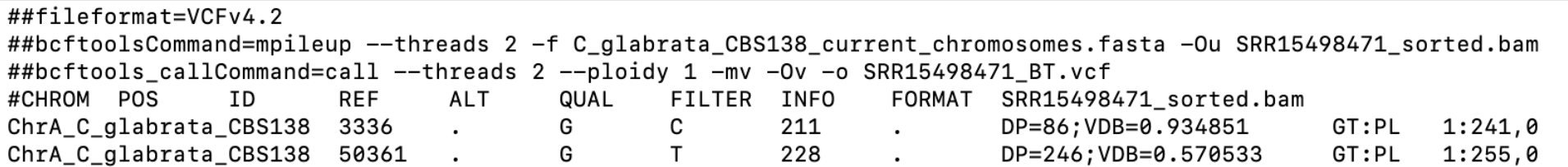
Fig. 5: An sample vcf file
Filtering Variants
Now that we’ve called our variants, we need to perform variant filtering – i.e. selecting certain variants based on specific criteria and parameters. This step can be quite tricky because there are many factors that influence variant calling and many different filters we can apply. In any case, to prepare the vcf file for filtering and other operations, we need to process it.
First, let's compress it and index the vcf file with the two following commands:
bgzip -c SRR15498471_FB.vcf > SRR15498471_FB.vcf.gz
tabix -p vcf SRR15498471_FB.vcf.gz
Now we can filter our variants with the following command:
bcftools filter -Oz -o SRR15498471_FB_filtered.vcf.gz -i 'QUAL>20 && INFO/DP>100' SRR15498471_FB.vcf.gzLet’s explore this command before moving on.
QUAL>20 tells bcftools to keep only variants with a quality score greater than 20.
DP>100 keeps only variants with read depth greater than 100.
INFO tells bcftools that we want to filter the DP information specifically from the INFO column (we need to specify this because freebayes writes the DP parameter in both INFO and FORMAT columns)
Again, filtering vcf files is quite complex because there can be various technical and biological factors biasing variant calling results. The command above is only one illustrative example.
Indexing & Checking the VCF
Now that we’ve filtered our vcf file, let’s index it with this command:
tabix -p vcf SRR15498471_FB_filtered.vcf.gzFinally, we can do a quick comparison of the filtered and original vcf files. Let's run these commands:
bcftools view SRR15498471_FB.vcf.gz | grep -v "#"| wc -l
bcftools view SRR15498471_FB_filtered.vcf.gz | grep -v "#"| wc -l
The above commands open the gzipped vcf files with bcftools, exclude metadata and header lines starting with # sign (grep -v “#”) and then simply count the number of lines. They should output the values 1439 and 312, respectively. In other words, filtering has reduced the number of variants from 1439 to 312.
Variant Calling with bcftools
Runtime: 5 minutes on the Workstation, 12 minutes on the Mac
Now we will perform variant calling with another popular program called bcftools. Bcftools is very versatile software, and it can be used to manipulate vcf files in complex ways. (For example, we already used it to perform variant filtering in the previous step.)
Let’s run bcftools for variant calling with the following set of commands:
bcftools mpileup --threads 2 -f ../ref_gen/C_glabrata_CBS138_current_chromosomes.fasta SRR15498471_sorted.bam -Ou | bcftools call --threads 2 --ploidy 1 -mv -Oz -o SRR15498471_BT.vcf.gzBefore we move on, let's explore how this command works:
First, bcftools performs the mpileup operation, which calculates genotype likelihoods from our mapped data. Then bcftools call will actually perform the variant calling and output vcf files. In the mpileup process, --threads 2 tells bcftools to use 2 processor cores, while -Ou instructs the software to operate in bcf mode (i.e. compressed vcf, which saves time for calculations). The --ploidy option specifies that our data is haploid, -mv are options related to the algorithm of variant calling, and -Oz tells bcftools to output the result file in a gzipped vcf. When finished, we will get a file called SRR15498471_BT.vcf.gz.
Now let’s index and filter that file using these commands:
tabix -p vcf SRR15498471_BT.vcf.gz
bcftools filter -Oz -o SRR15498471_BT_filtered.vcf.gz -i 'QUAL>20 && DP>100' SRR15498471_BT.vcf.gz
And now let’s index the resulting filtered file using this command:
tabix -p vcf SRR15498471_BT_filtered.vcf.gzFinally, let's have a look at how the filtering has affected our results. Run these commands:
bcftools view SRR15498471_BT.vcf.gz | grep -v "#"| wc -l
bcftools view SRR15498471_BT_filtered.vcf.gz | grep -v "#"| wc -l
These commands should output results of 322 and 201, respectively. This tells us that filtering has reduced our variant count from 322 to 201.
Intersecting Results from Two Variant Calling Procedures
In the two previous sections, we obtained filtered vcf files from both bcftools and freebayes software. Now we’ll select the variants which are detected by both programs for downstream analysis. With this approach, we increase our chances of obtaining real variants and minimize potential false positives. For this step, we will again use bcftools, but now with the isec (i.e. intersect) option.
To begin, run the following command:
bcftools isec -p isec_dir SRR15498471_BT_filtered.vcf.gz SRR15498471_FB_filtered.vcf.gzThis command will create a folder called isec_dir, which contains the following vcf files:
- 0000.vcf – variants exclusive to SRR15498471_BT_filtered.vcf.gz
- 0001.vcf – variants exclusive to SRR15498471_FB_filtered.vcf.gz
- 0002.vcf – variants from SRR15498471_BT_filtered.vcf.gz shared by both vcf files
- 0003.vcf – variants from SRR15498471_FB_filtered.vcf.gz shared by both vcf files
In essence, we have now identified variants which are unique to either of our vcf files (i.e. 0000.vcf and 0001.vcf), and variants which are shared between both files (i.e. 0002.vcf and 0003.vcf). Note that, as expected, 0002.vcf and 0003.vcf have the same number of variants (76 – run for example bcftools view 0003.vcf | grep -v "#"| wc -l to see this). Even so, we created both files because bcftools and freebayes have different types of metadata and column formatting. That allows us to choose the final vcf file depending on which format we prefer for downstream analysis. We will move forward with the file 0002.vcf (which is in bctools mpileup/call output formats). For simplicity, let’s copy and rename that file using this command:
cp new_dir/0002.vcf final_intersect_variants.vcfTo summarize this section, we have now performed variant calling and filtering with two popular software packages – bcftools and freebayes – and obtained high-confidence variants by identifying the intersection of results produced by both programs. In the following sections, we will visualize our variant calling data and perform its annotation.
Visualizing SNP/Variant Calling Data
Runtime: Depends on how long you spend investigating the data
If you’re trying to develop a deeper and more intuitive understanding of NGS data, visualization is a powerful option. In this step, we are going to visualize all the results that we have obtained so far. We will first look at the bam read alignment file and visually inspect the variants that we obtained during the previous step of variant calling. To do so, we will use Integrative Genomics Viewer (IGV).
First, let's install this software in our varcall environment:
conda install igv --channel conda-forge --channel bioconda --strict-channel-priorityNow launch IGV with this command:
igvThis will open a graphical user interface for the program. Go to Genome > Load Genomes from File > select the genome fasta file of C. glabrata. The chromosomes of the yeast will appear at the top of IGV. Now go to File > Load from file > select the gff annotation file of C. glabrata. The genome annotations will appear underneath the chromosome, showing genes and other annotated elements of the genome. We can right-click on the annotations track, and select “Expanded” option to see all features clearly. Next, go to File > Load from file > select the indexed bam file SRR15498471_sorted.bam. Then, go to File > Load from file > select the final variants final_intersect_variants.vcf.
Now that all files are loaded, let's try to find some of the variants and take a closer look. For example, select the first chromosome of C. glabrata from the drop-down menu (i.e. ChrA_C_glabrata_CBS138), and zoom in on the only variant found on that chromosome (the blue band at the top track). If we zoom in (using the + sign at top-right corner), we can see a clear single nucleotide polymorphism (SNP) which changes the reference G to T. We also can see (Fig. 6) that this SNP is located within a gene called PDR1 (CAGL0100451g):
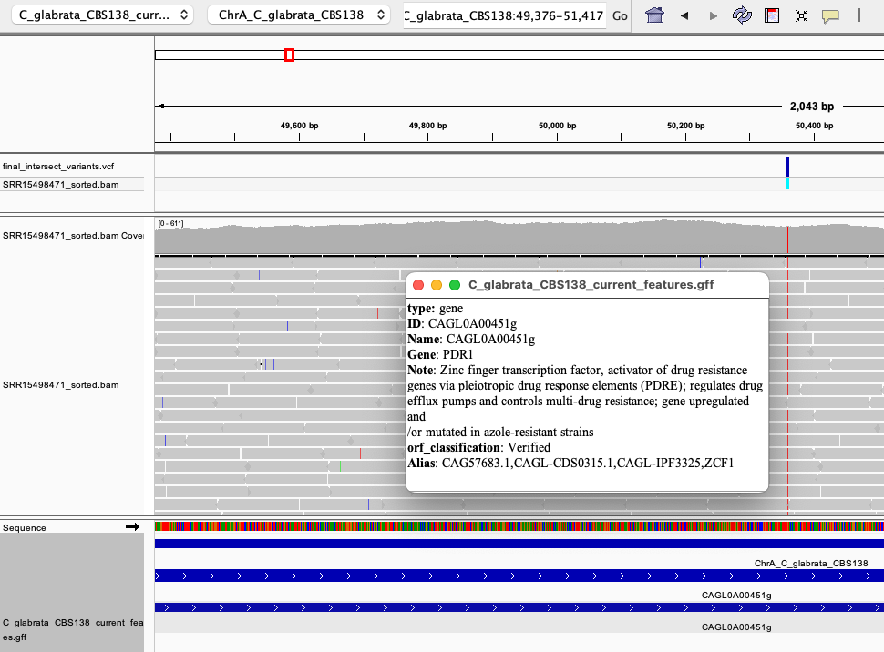
Fig. 6: A SNP detected in the PDR1 - a gene directly involved in the emergence of drug resistance in C. glabrata.
This reveals that we hit the bullseye, because mutations in PDR1 are notorious for causing drug resistance in C. glabrata (Tsai et al. 2006, Fardeau et al. 2007). PDR1 is a transcription factor that regulates the expression of efflux pumps (proteins that can spit out drugs from the fungal cell). Usually mutations in PDR1 lead to its overexpression which highly activates the efflux of drugs from this yeast, turning it into drug-resistant pathogen. Here, we have essentially confirmed that fluconazole-resistant C. glabrata has a point mutation in PDR1.
However, there are other mutations in our C. glabrata data which are less obviously related to drug resistance than the PDR1 variant. Some of these are located in intergenic regions (Fig. 7) or within other genes:
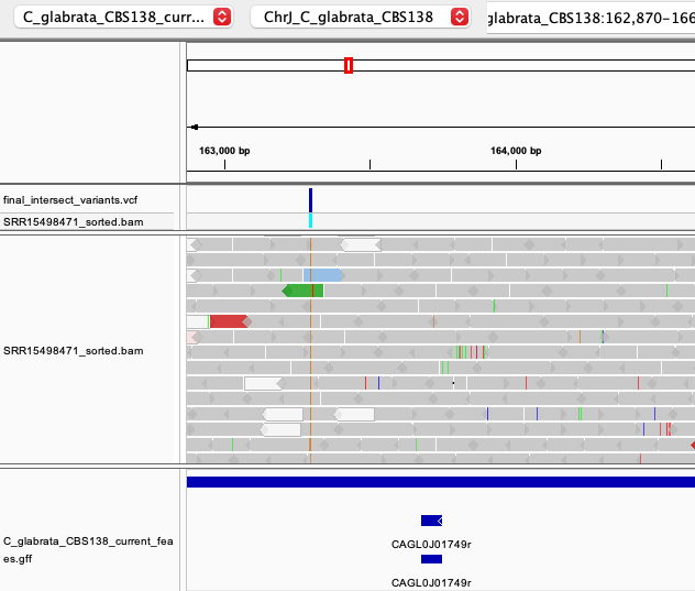
Fig. 7: An example of intergenic SNP on chromosome J.
Although visualization in IGV is very useful for manually inspecting a small number of mutations, we need a more general approach to systematically characterize our variant calling data. That is why the next (and final) step of this tutorial delves into variant annotation.
SNP/Variant Annotation Workflow
Runtime: Less than a minute on both computers
We have come to the final step of our tutorial – variant annotation. Variant annotation is a technique to systematically characterize variants. It can tell us what type of variants we have (SNPS, indels, inversions, etc.), in which genomic regions they appear (intergenic, genic, UTRs, etc.), whether they are synonymous or non-synonymous, what type of amino-acid changes they cause, and much more.
For this step, we will use a software package called SnpEff that can perform variant annotation and predict functional effects of variants on genes and proteins. Note that SnpEff is very powerful and versatile. In this tutorial, we are only covering its main functionalities related to variant annotation.
First, install SnpEff via Conda using the following command:
conda install snpeff --channel conda-forge --channel bioconda --strict-channel-priorityTo perform the annotation of our final variants, simply run:
snpEff Candida_glabrata final_intersect_variants.vcf > snpEff_report.vcfNote: SnpEff has a very large database of organisms which it uses to annotate variants of interest. C. glabrata (which we specified in the command) is one of those organisms.
Upon finishing, SnpEff outputs three files: genes.txt, summary.html, and report.vcf (which we specified in the command above). Let's open the summary.html report using a web browser. As you can see, this is a very comprehensive report that describes many different parameters of our variants – e.g., their distribution per chromosome and per feature (gene, exon, intron, UTR, integenic, etc.), types of variants, types of base/codon/amino acid changes, and much more.
For example, let’s look at the plot for predicted functional effects of variants:
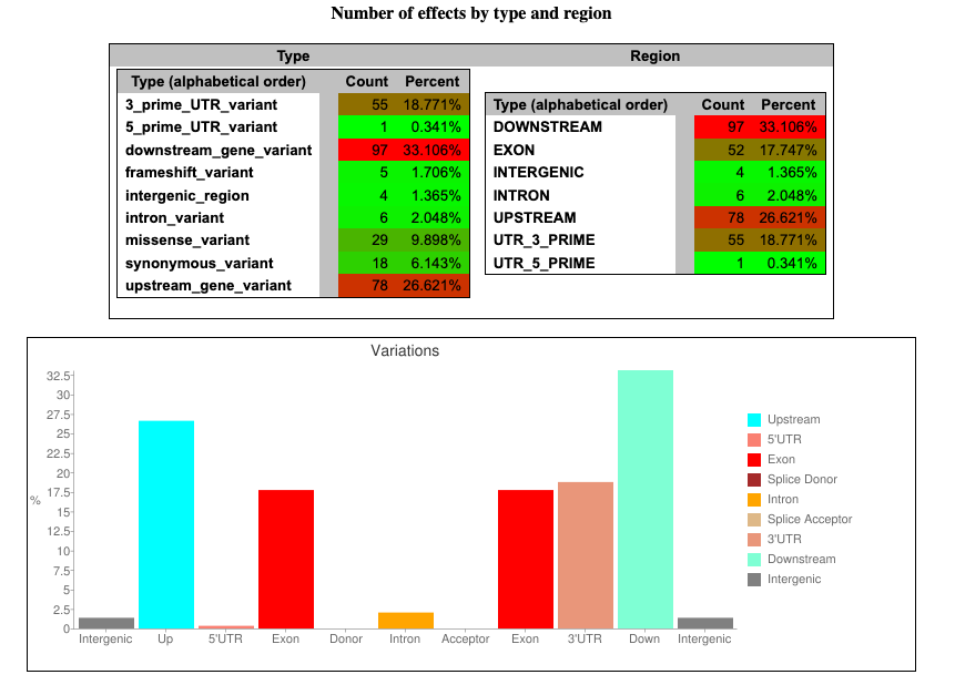
Fig. 8: An example plot from an SnpEff report on the number of possible variant effects by type and region.
In this plot, we can see (for example) that most of the potential effects (33.1%) are related to the mutations in downstream regions of genes.
Now let's examine the file snpEff_gene.txt produced by SnpEff. This file contains information about the variants located in genomic regions. It has 16 columns, the first 4 of which are about the gene. The remaining 12 display the number of variants and possible variant effect types that each gene harbors (low impact, high impact, missense variants, etc.). For example, we can see (Fig. 9) that the PDR1 gene that we saw above has one missense variant with moderate impact, meaning that it changes the amino acid of the protein.
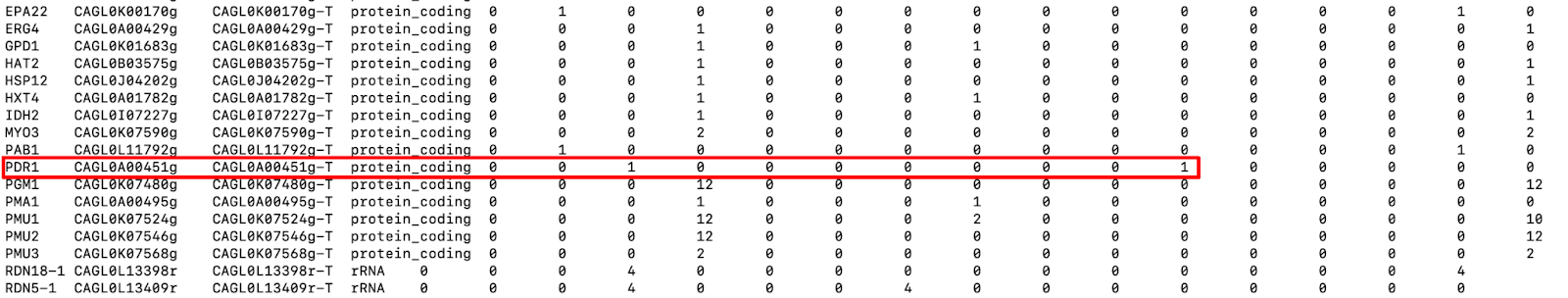
Fig. 9: A snapshot of snpEff_gene.txt file. Red rectangle highlights the mutations in the PDR1 gene.
Note that SnpEff assesses the possible effects of variants using Sequence Ontology. You can learn more here about how the software predicts possible effects and their impacts (low, high, etc). Bear in mind that these impact categories were created only to simplify the filtering process of the data. There is no way to predict whether a "high impact" or a "low impact" variant is the one producing a particular phenotype. For example, the mutation in PDR1 was only labeled “moderate impact,” but we know from numerous sources of experimental evidence that mutations in PDR1 are actually the direct cause of drug resistance in C. glabrata.
Finally, let’s have a look at the vcf file snpEff_report.vcf. It appears largely similar to our initial vcf file with filtered variants, except that SnpEff has added a lot of information in the INFO column for each variant (along with some metadata lines). Now each variant has additional annotation (ANN) in the INFO columns, which have 16 fields separated by the “|” sign.
Here are the 16 fields:
- Allele
- Annotation (a.k.a. effect)
- Putative_impact
- Gene Name
- Gene ID
- Feature type
- Feature ID
- Transcript biotype
- Rank / total
- HGVS.c (see here)
- HGVS.p (see here)
- cDNA_position / cDNA_len
- CDS_position / CDS_len
- Protein_position / Protein_len
- Distance to feature
- Errors, Warnings or Information messages
(Learn more here about these fields.)
Note that a given variant will have several annotations if it affects several genomic elements – e.g. if a variant is harbored by two genes at the same locus but on opposite DNA strands.
Using the example of the variant in the PDR1 gene, let’s explore the annotation made by SnpEff. The software has inferred that the variant G>T located in PDR1 at chromosomal position 50361 can potentially affect 4 genes – the PDR1 itself, two downstream genes CAGL0A00495g and CAGL0A00473g, and one upstream gene CAGL0A00429g (also known as ERG4, which is also implicated in fluconazole resistance in this yeast). For each potentially affected gene, SnpEff produces the corresponding annotations below. (In the vcf files, all of these annotations are written in one line.)
- ANN=T|missense_variant|MODERATE|PDR1|CAGL0A00451g|transcript|CAGL0A00451g-T|protein_coding|1/1|c.2805G>T|p.Leu935Phe|6059/6884|2805/3324|935/1107||,
- T|upstream_gene_variant|MODIFIER|ERG4|CAGL0A00429g|transcript|CAGL0A00429g-T|protein_coding||c.-6331C>A|||||3245|,
- T|downstream_gene_variant|MODIFIER|CAGL0A00473g|CAGL0A00473g|transcript|CAGL0A00473g-T|protein_coding||c._776C>A|||||674|,
- T|downstream_gene_variant|MODIFIER|PMA1|CAGL0A00495g|transcript|CAGL0A00495g-T|protein_coding||c._4653C>A|||||3327|
Having this detailed information about every single variant opens many opportunities for exploring the obtained data – and further performing more targeted experiments to investigate the question of interest. In our case, for example, investigators could try to experimentally introduce or remove the newly found variants into C. glabrata to determine whether some of them are causal variants for drug resistance.
To summarize this section, we have annotated our high-confidence variants using SnpEff software, which gave us very comprehensive and detailed information about each observed variant.
Background: What is Variant/SNP Calling?
Recent advances in Next-Generation Sequencing (NGS) have helped us decode the genomes of thousands of living and extinct species. This has opened the door for deeper DNA analysis, as researchers delve into each decoded species and explore genomic variations between individuals. Thanks to this work, we're seeing exciting new answers to long-standing scientific questions in the fields of medicine, evolutionary biology, ecology, and more.
At the core of this study of genomic variation is variant calling. Variant calling is the process of comparing an organism’s genome sequence to a reference sequence for its species, so that we can identify single-nucleotide polymorphisms (SNPs) and small insertions and deletion (indels).
Note that there are other types of genomic variation, such as structural variants (SV), which involve larger genomic changes (from >50 bp up to whole chromosomes). The analysis of SVs is quite complex and thus is not covered in this guide.
Variant calling analysis is a powerful and flexible technique. It produces results that are used for everything from phylo- and population genomics to biotechnology and precision medicine. In this guide, we’ll use it to examine the genome of a common pathogenic yeast and identify genes related to its drug resistance.
Variant Calling/SNP Calling Experimental Design
When you’re performing a scientific experiment, good experimental design (aka study design) is essential. Fortunately for us, variant calling projects are relatively simple in design – unlike RNA-Seq, ATAC-Seq, and other techniques that deal with highly dynamic biological systems. This is because variants are typically more stable than, for example, expression levels and are not often affected by the short-term treatments/experimental manipulations that can impact expression levels. (See the section on Experimental Design in our RNA-Seq guide for more insights.) This mean that variant-calling projects do not suffer from issues like batch effects to the same extent that RNA-Seq projects do.
Nevertheless, there are several factors you should always account for when designing your variant calling experiment. We’ll explore them in the following sections.
DNA Isolation & Fragmentation For Variant/SNP Calling
When you isolate DNA from a biological sample, the isolation method you choose can have systemic effects on the representation of different genomic regions. This can impact downstream analyses like variant detection (Zverinova and Guryev, 2022, van Heesch, et al, 2013). Additionally, DNA fragmentation – which is necessary to prepare a sequencing library – can influence your variant calling results.
To safeguard against these potential distortions in your data, we strongly recommend using the same DNA isolation and library preparation protocols for all analyzed samples within a single project. If that is not possible (for instance, because you’re analyzing publicly available data from different projects), it is at least advisable to know which protocols were used for each project/sample.
In this tutorial, we will analyze C. glabrata yeast data from a study by Ksiezopolska et al (2021) which used the same DNA extraction method (Master Pure Yeast DNA purification kit) for all samples.
Genome Coverage and Read Length
To perform reliable variant calling, we first need to obtain sufficient read data. In other words, our genome coverage needs to be adequate. Genome coverage is a metric that indicates how many times each nucleotide in an analyzed genome is covered by reads. For example, 30x coverage (which is generally considered a satisfactory coverage level) means that each nucleotide in the genome is covered by (on average) 30 reads. It can be calculated by a simple formula:
Coverage = (Number of reads* Read length ) / Total genome size
Using this formula, you can easily derive how many reads you should sequence to achieve your desired coverage level:
Number of reads = (Coverage* Total genome size) / Read length
However, it’s important to note that the resulting number of reads does not guarantee uniform coverage across all genomic loci, because some reads may not map to the genome. There may also be deletions, duplications, and other factors which can influence the final coverage of the data. In other words, this formula is only a rough approximation to help you target a sequencing depth and budget your experiment.
The target read length may vary, depending on your specific experiment and the organism you’re studying. Longer reads tend to map better than shorter ones, and so are generally recommended. However, a short read may be sufficient if an organism has low genomic complexity (e.g. its genome contains few repetitive regions). As a rule, paired-end sequencing is recommended over single-end sequencing.
The most popular sequencing technology (“Sequencing-by-Synthesis” by Illumina Inc.) offers read lengths ranging from 50 to 300 base pairs. Because it supports high-coverage sequencing, this is the primary technology used for variant calling analysis today.
PCR Duplicates
PCR duplicates are redundant reads that originate from the same DNA fragment. They are produced during the PCR amplification step of library preparation. In theory, these artifacts can falsely increase allele frequency or introduce erroneous mutation to the data.
PCR duplicates can be avoided by using modern, PCR-free library preparation protocols. In the absence of these protocols, you can still remove or mark PCR duplicates bioinformatically. However, a recent report showed that removal/marking of these duplicates largely does not affect the variant calling results
Summary
In this end-to-end tutorial we have covered the major steps of variant calling analysis, using the whole-genome sequencing data of a drug-resistant human fungal pathogen C. glabrata. The techniques we used are very versatile and powerful, and can be used for many other real-world projects. That said, some aspects of variant calling analysis (such as variant filtering, annotation, and interpretation) can be quite specific for a given experiment or organism. There is no one-size-fits-all method in bioinformatics, and you may have to adapt these methods significantly for your own project.
We do hope that this guide makes variant calling more clear, intuitive, and accessible for everyone. If there are ways we can improve it, please let us know! We’d love to hear your feedback.
References
- Cingolani, Pablo, Adrian Platts, Le Lily Wang, Melissa Coon, Tung Nguyen, Luan Wang, Susan J. Land, Xiangyi Lu, and Douglas M. Ruden. 2012. “A Program for Annotating and Predicting the Effects of Single Nucleotide Polymorphisms, SnpEff: SNPs in the Genome of Drosophila Melanogaster Strain w1118; Iso-2; Iso-3.” Fly 6 (2): 80–92. https://doi.org/10.4161/fly.19695
- Ebbert, Mark T. W., Mark E. Wadsworth, Lyndsay A. Staley, Kaitlyn L. Hoyt, Brandon Pickett, Justin Miller, John Duce, Alzheimer’s Disease Neuroimaging Initiative, John S. K. Kauwe, and Perry G. Ridge. 2016. “Evaluating the Necessity of PCR Duplicate Removal from next-Generation Sequencing Data and a Comparison of Approaches.” BMC Bioinformatics 17 Suppl 7 (July): 239. https://doi.org/10.1186/s12859-016-1097-3
- Ewels, Philip, Måns Magnusson, Sverker Lundin, and Max Käller. 2016. “MultiQC: Summarize Analysis Results for Multiple Tools and Samples in a Single Report.” Bioinformatics 32 (19): 3047–48. https://doi.org/10.1093/bioinformatics/btw354
- Fardeau, V., G. Lelandais, A. Oldfield, H. N. Salin, S. Lemoine, M. Garcia, V. Tanty, S. Le Crom, C. Jacq, and F. Devaux. 2007. “The Central Role of PDR1 in the Foundation of Yeast Drug Resistance.” The Journal of Biological Chemistry 282 (7). https://doi.org/10.1074/jbc.M610197200.
- Garrison, Erik, and Gabor Marth. 2012. “Haplotype-Based Variant Detection from Short-Read Sequencing,” July. https://doi.org/10.48550/arXiv.1207.3907.
- Heesch, Sebastiaan van, Michal Mokry, Veronika Boskova, Wade Junker, Rajdeep Mehon, Pim Toonen, Ewart de Bruijn, et al. 2013. “Systematic Biases in DNA Copy Number Originate from Isolation Procedures.” Genome Biology 14 (4): R33. https://doi.org/10.1186/gb-2013-14-4-r33
- Ksiezopolska, Ewa, Miquel Àngel Schikora-Tamarit, Reinhard Beyer, Juan Carlos Nunez-Rodriguez, Christoph Schüller, and Toni Gabaldón. 2021. “Narrow Mutational Signatures Drive Acquisition of Multidrug Resistance in the Fungal Pathogen Candida Glabrata.” Current Biology: CB 31 (23): 5314–26.e10. https://doi.org/10.1016/j.cub.2021.09.084
- Li, Heng. 2011. “A Statistical Framework for SNP Calling, Mutation Discovery, Association Mapping and Population Genetical Parameter Estimation from Sequencing Data.” Bioinformatics 27 (21): 2987–93. https://doi.org/10.1093/bioinformatics/btr509
- Li, Heng, and Richard Durbin. 2009. “Fast and Accurate Short Read Alignment with Burrows-Wheeler Transform.” Bioinformatics 25 (14): 1754–60. https://doi.org/10.1093/bioinformatics/btp324
- Robinson, James T., Helga Thorvaldsdóttir, Wendy Winckler, Mitchell Guttman, Eric S. Lander, Gad Getz, and Jill P. Mesirov. 2011. “Integrative Genomics Viewer.” Nature Biotechnology 29 (1): 24–26. https://doi.org/10.1038/nbt.1754
- Skrzypek, M. S., J. Binkley, G. Binkley, S. R. Miyasato, M. Simison, and G. Sherlock. 2017. “The Candida Genome Database (CGD): Incorporation of Assembly 22, Systematic Identifiers and Visualization of High Throughput Sequencing Data.” Nucleic Acids Research 45 (D1). https://doi.org/10.1093/nar/gkw924.
- Tsai, H. F., Krol, A. A., Sarti, K. E., & Bennett, J. E. (2006). Candida glabrata PDR1, a transcriptional regulator of a pleiotropic drug resistance network, mediates azole resistance in clinical isolates and petite mutants. Antimicrobial agents and chemotherapy, 50(4), 1384–1392. https://doi.org/10.1128/AAC.50.4.1384-1392.2006
- Zverinova, Stepanka, and Victor Guryev. 2022. “Variant Calling: Considerations, Practices, and Developments.” Human Mutation 43 (8): 976–85. https://doi.org/10.1002/humu.24311
Updated 5 months ago