RNA-Seq Differential Expression Tutorial (From Fastq to Figures)
Go to ai.tinybio.cloud/chat to chat with a life sciences focused ChatGPT.
This end-to-end tutorial will guide you through every step of RNA-Seq data analysis. We’ll show you how to set up your computing environment, fetch the raw sequencing data, perform read mapping, peak calling, and differential accessibility analysis, and finally visualize and interpret the results.
All you need is a reasonably modern desktop/laptop computer with a Linux/Unix-like operating system and some basic knowledge of bash and R scripting.
This tutorial primarily focuses on the bioinformatics portion of the RNA-Seq Analysis. The background and overview can be found here. For highlights of the tutorial, see the below:
- Trimming RNA-Seq Fastq Samples
- RNA-Seq Read Quantification
- RNA-Seq Read Mapping
- RNA-Seq Differential Gene Expression Analysis
- GO Term Enrichment Analysis
Create a Computing Environment
This tutorial will require a number of different software packages that need to interact smoothly. To download and install them, we’ll use Conda – a free package management system. (Learn more about Conda in our detailed guide.)
To begin, download and install Miniconda (a minimal Conda installer) if you haven’t already. When Conda is available, we’ll create and activate an environment called rnaseq. In your terminal, type:
conda create -n rnaseq
conda activate rnaseq
Next, let's configure our Conda channels with the following commands:
conda config --add channels defaults
conda config --add channels bioconda
conda config --add channels conda-forge
conda config --set channel_priority strict
We have now set up our computing environment and can move on to the next step. For the rest of this tutorial, we’ll use Conda to download and manage software on the go.
RNA-Seq Data Analysis: A Quick Overview
In this tutorial, we will analyze the RNA-Seq data of the human pathogenic yeast C_andida parapsilosis_.
C. parapsilosis is one of the major opportunistic fungal pathogens. It can cause a life-threatening systemic infection known as candidiasis, with mortality rates reaching 25 percent. This yeast can grow in two different morphological states – a non-pathogenic planktonic form, and a pathogenic form called a biofilm, in which yeast cells form tightly interconnected structures.
In this tutorial, we will analyze the RNA-Seq data of C. parapsilosis in these two states. Our goal is to reproduce the results of a study by Holland and colleagues, 2014, which used RNA-Seq to perform a differential gene expression analysis of C. parapsilosis, thus identifying genes and pathways implicated in the formation of biofilms of this species.
Specifically, the study assessed three biological replicates of C. parapsilosis in each of the two states (planktonic and biofilm). The samples were prepared with a strand-specific library preparation protocol and subsequently sequenced using an Illumina HiSeq 2000 device with paired-end 2x90 bp read-length. All samples were sequenced for ~13 million paired-end reads, which is quite abundant for differential gene expression analysis in a yeast.
RNA-Seq Data Pipeline
In this tutorial, we’ll run our data through a multi-stage RNA-Seq data analysis pipeline. Here is a simplified schematic of our workflow:
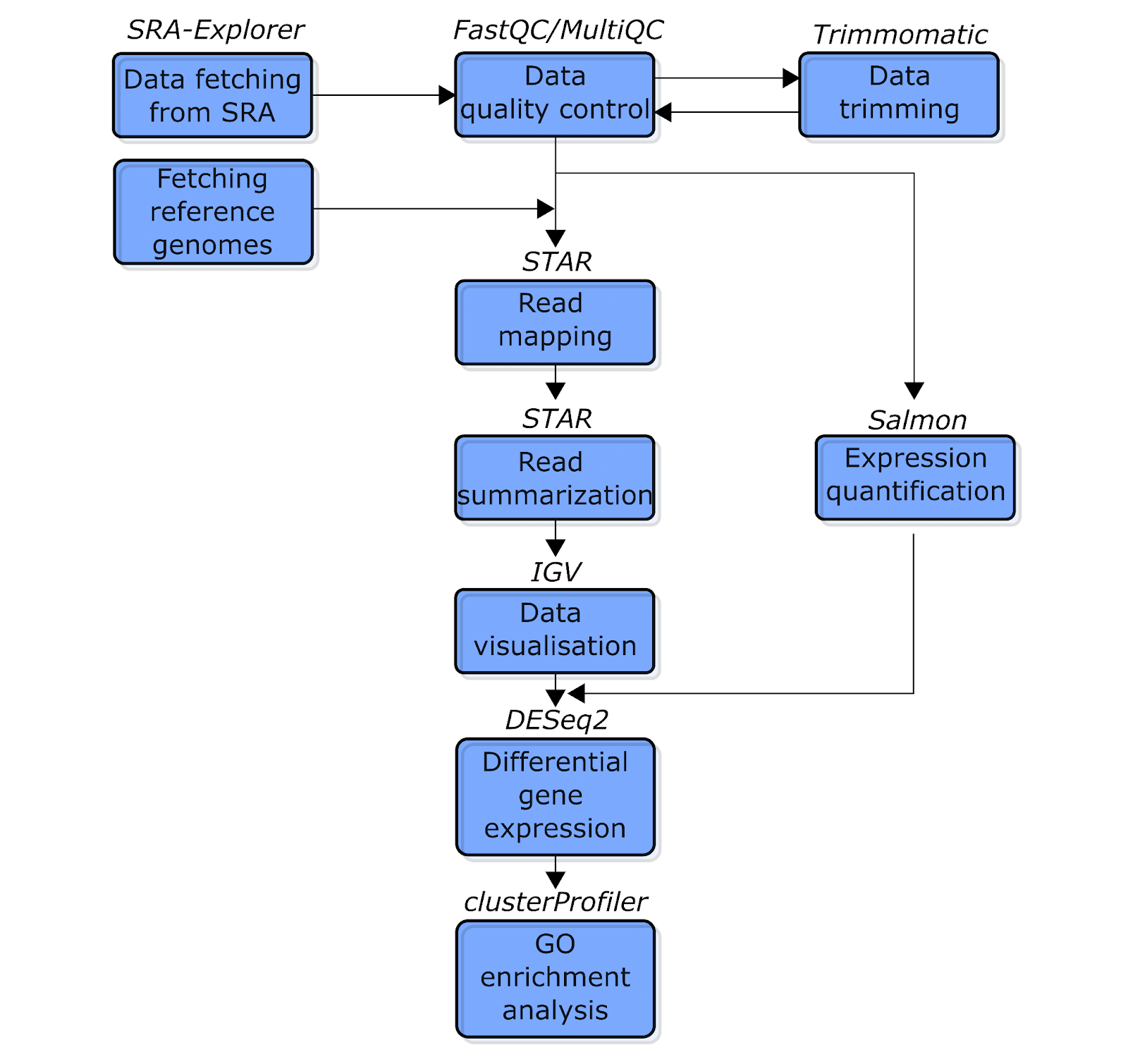
Fig. 1: The simplified schematic flowchart of the RNA-Seq data analysis pipeline covered in this tutorial. Blue boxes indicate the types of analysis. The text above the boxes indicates the software used for each analysis.
Let’s briefly explore the stages of this workflow before we begin:
First, we will download the data from Sequence Read Archive (SRA) using SRA Explorer. Then, as in other NGS data analysis workflows, we will run a quality control analysis before proceeding with the main analysis. We will perform this step using FastQC and MultiQC (Ewels et al. 2016) software. Next, we will use Trimmomatic (Bolger, Lohse, and Usadel 2014) software to remove reads with poor quality.
Once our data is cleaned, we will use two different methods to quantify read counts for each gene. First, we will perform a “classical” read mapping to reference the genome using STAR software (Dobin et al. 2013), which will generate sequence alignment files (sam/bam files). We will also use STAR to count the number of reads mapped to each gene. Second, we will use Salmon (Patro et al. 2017) to conduct a so-called pseudo/quasi-mapping approach. This is a lightweight and very fast technique to quantify reads per transcript/gene, bypassing the step of sam/bam file generation. (For a more detailed comparison of these methods, see the corresponding sections.)
Next, our obtained read count data will be loaded to R to perform differential gene expression analysis using the DESeq2 Bioconductor package (Love et al. 2014). We will also visualize the obtained results in this step. Finally, we will use the clusterProfiler Bioconductor package (Yu et al. 2012) to perform GO term enrichment analysis of up-regulated genes in the biofilm condition. This will reveal which biological processes are implicated in biofilm formation in C. parapsilosis.
RNA-Seq Environment Activation
Before we move on, be sure you've set up a computing environment using Conda. If you haven't already, activate the rnaseq conda environment now by running this command:
conda activate rnaseqHardware Requirements
You can complete this tutorial using any reasonably modern laptop or desktop computer with a Linux/Unix-like operating system. Of course, some steps require a lot of processing and thus will execute faster on more powerful machines. We'll share approximate run-times for each step, so you can estimate how long it might take on your own computer. These are the two devices we used to test this tutorial:
-
Workstation – a desktop computer with Intel Core i7-8700K CPU, 3.70GHz, and 64 GB of RAM running on Open-Suse Leap 15.3
-
Mac – a 2017 MacBook Pro with 2.3 GHz Dual-Core Intel Core i5 and 8 GB of RAM, running on MacOs Monterey 12.4.
Processing our data will require no more than 8 GB of RAM at any point, thanks to the small size of the yeast reference genome which the data will be mapped to. This end-to-end RNA-Seq analysis can thus be performed on any modern desktop/laptop computer. See the steps below for approximate run times.
The entire analysis requires ~35 GB of hard drive space, although certain large files (such as fastq or bam files) can be removed after the read mapping step.
File System
To keep your RNA-Seq analysis cleanly organized, we recommend creating the following folders in any convenient directory:
- raw_data
- raw_data/trimming
- ref_gen
- mapping
To create these directories, run the following command:
mkdir -p ./ref_gen/ ./mapping ./raw_data/trimmingWe will create other folders on the go during this tutorial. But to get started, we only need the four folders listed above.
Data Fetching
Run time: Depends on internet connection speed. For 50 Mbps, this step takes ~4 minutes.
To perform our RNA-Seq analysis, we first need to obtain a suitable data set. We will fetch this data using SRA Explorer – an online tool for efficiently searching and downloading raw sequencing data.
Go to SRA Explorer and enter the project accession number PRJNA246482, which corresponds to the study we’re reproducing by Holland et al, 2014. Then select the first six SRR accession number entries (i.e. SRR1278968 through SRR1278973), and add them to the collection. Then go to saved datasets, and download the Bash script for downloading FastQ files. Now locate the downloaded file sra_explorer_fastq_download.sh in the raw_data folder and go to that folder using this command:
cd raw_data/By default, SRA Explorer commands will rename the downloaded files. In our case, this is unnecessary. To prevent the renaming, run this command:
sed "s/GSM.\*Seq\_//g" sra_explorer_fastq_download.sh > renamed_sra_explorer.shThe sed command above will simply drop the unnecessary text from the file names. It removes any text starting with “GSM” and ending with “Seq_”. After renaming, simply run the command below to download the sequencing data.
bash renamed_sra_explorer.shThe data will be downloaded in a compressed fastq format. When the process is finished, we need to create a file containing the file names of the samples. To do so, run this command:
ls SRR\*gz | cut -f 1 -d "\_" | sort | uniq > sample_ids.txtFor some downstream analyses (such as trimming, mapping, and pseudo-mapping), we will iterate over this file. This means we will read each line one by one, and run analyses for each sample.
RNA-Seq Sequencing Data Quality Control
Runtime: ~5 min on the Workstation, and ~12 min on the Mac
To prepare our raw sequencing data for downstream analysis, we first need to perform quality control. For this step, we’ll use FastQC software to discover important parameters of the data. Then we will aggregate the FastQC reports using MultiQC software. To begin, let’s install both software packages in our Conda environment. In the activated rnaseq environment in your terminal, type:
conda install fastqc multiqc --channel conda-forge --channel bioconda --channel defaults --strict-channel-priorityAfter FastQC and MultiQC are installed, create and select a directory called fastqc_initial using these commands:
mkdir ./fastqc_initial
fastqc *fastq.gz -o ./fastqc_initial -t 2
In this command, *fastqc.gzinstructs FastQC to analyze all files in the current directory that end with fastq.gz and store the results in the fastqc_initial directory. (The * wildcard sign is a regular expression that matches any characters of any length.) The-t 2 parameter instructs FastQC to use two cores of the computer. If more cores are available, you can choose a larger number to speed up the analysis.
Because FastQC reports the results for each fastq file separately, inspecting the results of many files can be tedious. For this reason, we will use the MultiQC tool to aggregate the results. Navigate to the fastqc_initial folder and run MultiQC:
cd ./fastqc_initial/
multiqc .
This command tells the software to search the current directory, pick the output files of FastQC, and make an aggregated html report of all samples. (Note that MultiQC can handle output from numerous other bioinformatics programs.)
Once the analysis is finished, open the generated report multiqc_report.html in your browser. The main results of the report should look like this:
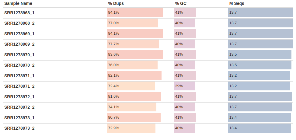
Fig. 2: The general statistics of the analyzed fastq samples, showing the sample names, duplication percentages, GC content percentages, and the number of sequencing reads.
Let’s review some features of this plot:
We can see that the rate of duplicated reads observed in our RNA-Seq data is relatively high. This is expected because highly-expressed genes can generate identical reads – especially in high-coverage data like ours.
The GC content – which is the percentage of G and C nucleotides over the total number of nucleotides – is ~39-41 percent. These are expected values for C. parapsilosis yeast.
Finally, the last column shows the numbers of sequenced reads. As mentioned above, each sample has ~13 million reads per each direction, which is more than enough for performing differential gene expression analysis for a yeast.
Next, let’s review the so-called Phred score for our data. Phred score is one of the main indicators of sequencing read quality. It indicates the reliability of each sequenced base, with values between 30 and 40 generally considered good scores. (Learn more here about Phred scores.) Scrolling down in the MultiQC report, you should see a plot of aggregated Phred scores across all samples at each base position:
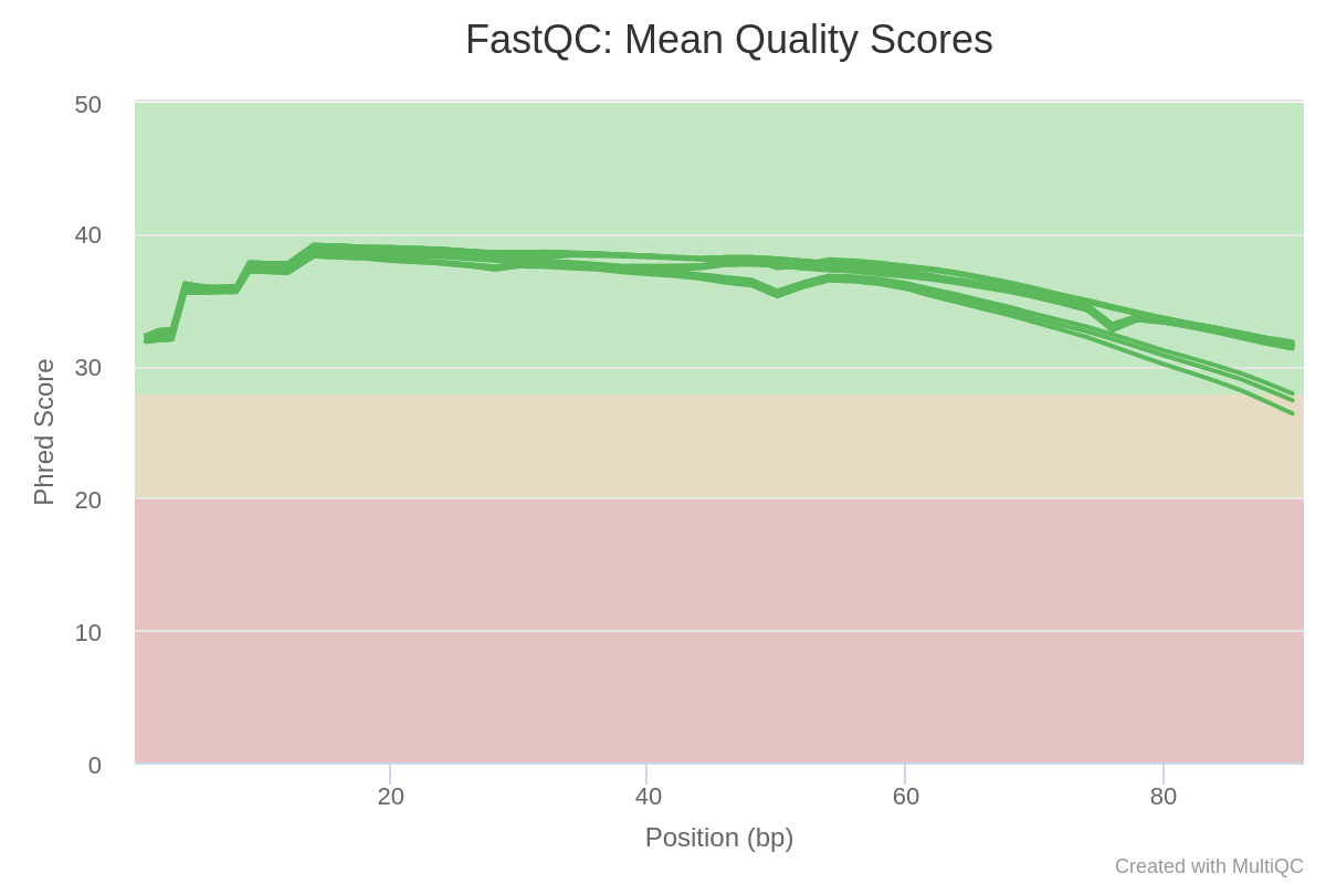
Fig. 3: Mean Phred-quality scores of each sample.
Notice that the quality of reads in all samples drops toward the end of the reads. In these situations, it is useful to investigate the original plots produced by FastQC. Unlike the aggregate MultiQC plot, they will show the quality scores using boxplots at every position, giving us more details about the data.
Now let’s look at the Phred scores for some specific samples. FastQC produces html reports, which can be viewed in any browser. Open the file SRR1278968_2.fastqc.html, which is the reverse read report for the sample SRR1278968. The plot should look like this:
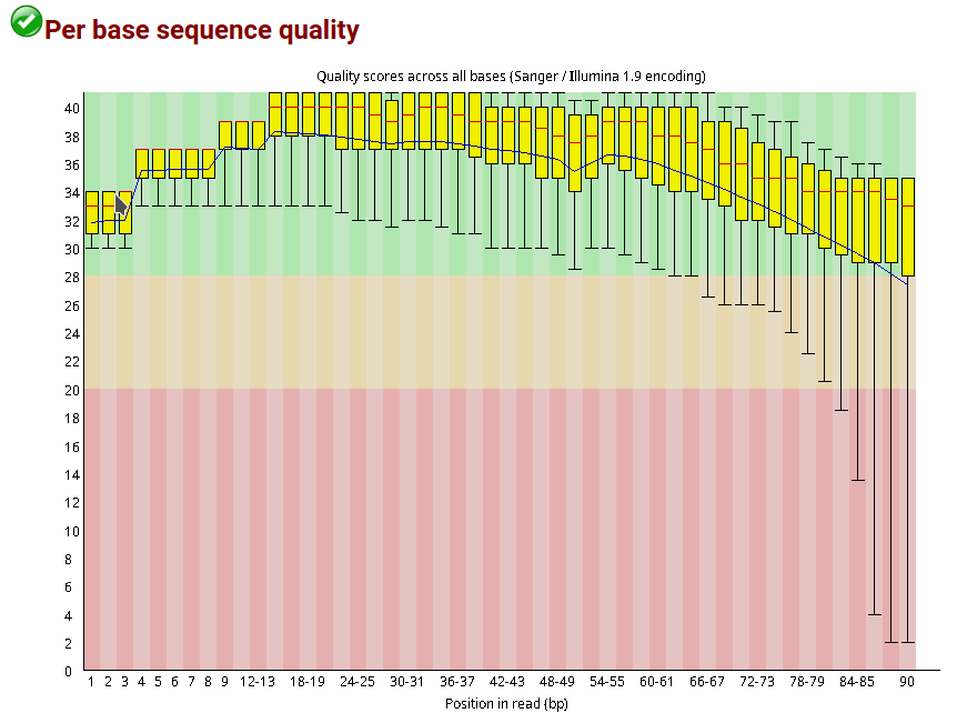
Fig. 4: Original FastQC report of Phred scores for the sample SRR1278968_2.fastqc.html
Here we can observe that Phred quality scores drop quite significantly at the end of the reads. You’ll notice that this same pattern appears in reverse reads of samples SRR1278968-SRR1278970. For our downstream analyses, we will need to remove these low-quality bases from our RNA-Seq data using a procedure called read trimming. (See the next section.)
Next, let’s check for the presence of adapter sequences which may have been introduced during the process of library preparation. As you can see in the “Adapter content” section of the report, no traces of adapter sequences were observed. When these sequences are found, it is important to trim them out – but in our case, that is not necessary. Hence, for the trimming step we will only need to remove the low-quality bases found by the plots above.
In summary, we have just run several quality control checks of our RNA-Seq data using the popular bioinformatics tools FastQC and MultiQC. Now that we’ve identified low-quality reads in our data, we’ll remove them in the next step of this tutorial.
Trimming RNA-Seq Fastq Samples
Runtime: ~30 minutes on the Workstation with 2 cores, ~1 hour on the Mac
In this section, we will trim our RNA-Seq data using the software Trimmomatic. Let's begin by installing this program in our rnaseq environment. First, run this command:
conda install trimmomatic --channel conda-forge --channel bioconda --channel defaults --strict-channel-priorityNow navigate to the raw_data/trimming folder:
cd ./trimmingTrimmomatic outputs four different files when trimming paired-end reads:
-
Forward-paired reads
-
Forward-unpaired reads
-
Reverse-paired reads
-
Reverse-unpaired reads.
The unpaired reads originate when one read of a pair survives trimming but the other does not. As a rule, only paired reads are used for the downstream analysis.
The following simple bash script
trimming.shwill generate Trimmomatic commands for each sample:
while read sample_id; do
echo trimmomatic PE -threads 2
../$sample_id_1.fastq.gz ../$sample_id_2.fastq.gz
$sample_id_tr_1P.fastq.gz $sample_id_tr_1U.fastq.gz\ $sample_id_tr_2P.fastq.gz
$sample_id_tr_2U.fastq.gz
LEADING:20 TRAILING:20 SLIDING WINDOW:4:20 MINLEN:50
done <../sample_ids.txt
This script iterates over the sample names contained in file **thesample_ids.txt** and generates a Trimmomatic command for each sample. Let’s break down the script a little further before moving on.

In the output files (for example ending with `tr_1P.fastq.gz`), “P” stands for “paired”, and “U” stands for unpaired, but you can specify any other names as you want. The parameters `LEADING:20` and `TRAILING:20` will remove bases with quality lower than 20 from the beginning and the end of the reads, respectively. The option `SLIDING WINDOW:4:20` will scan reads using a window of 4 bases and remove them if the average quality of these bases drops below 20. `MINLEN:50` will remove  reads shorter than 50 base pairs after the trimming.

Now let's generate the Trimmomatic commands. Just run this command:

```shell
bash trimming.sh > trimming_commands.txt
The command above creates a file called trimming_commands.txt which contains all commands for trimming. You can then run this file as a bash command or submit it as an array job in slurm/sge/other cluster schedulers. We’ll use this command:
bash trimming_commands.txt 1>trimming_output 2>trimming_errorThis will run the trimming commands. It will also redirect the standard output and standard error to corresponding files.
Now that we have trimmed our data, let’s confirm that our efforts were successful. First, we’ll create a new folder called fastqc_trimming. Use the following commands to check the trimmed data with FastQC and MultiQC:
mkdir fastqc_trimming
fastqc \*P.fastq.gz -o fastqc_trimming/ -t 2
multiqc .
MultiQC will now create another html report – but this one will contain results from Trimmomatic. As you can see, this report shows that on average 90% of paired-end reads survived the trimming:
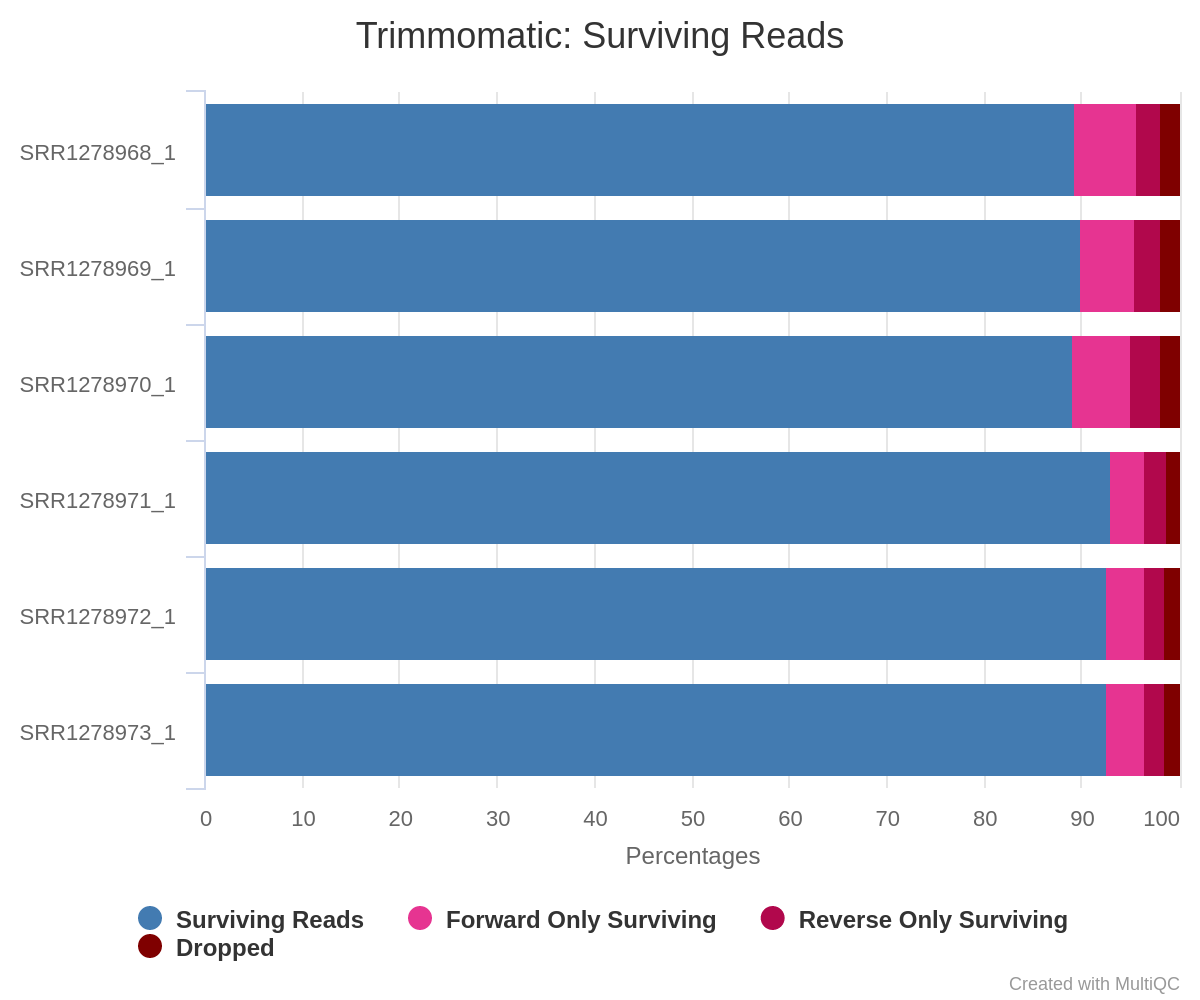
Fig. 5: Summary statistics of trimming results reported by MultiQC.
Finally, we can compare the Phred quality scores of the sample SRR1278968_2 before and after trimming (Fig. 6), which clearly demonstrates that low quality bases in the sample were removed after trimming.
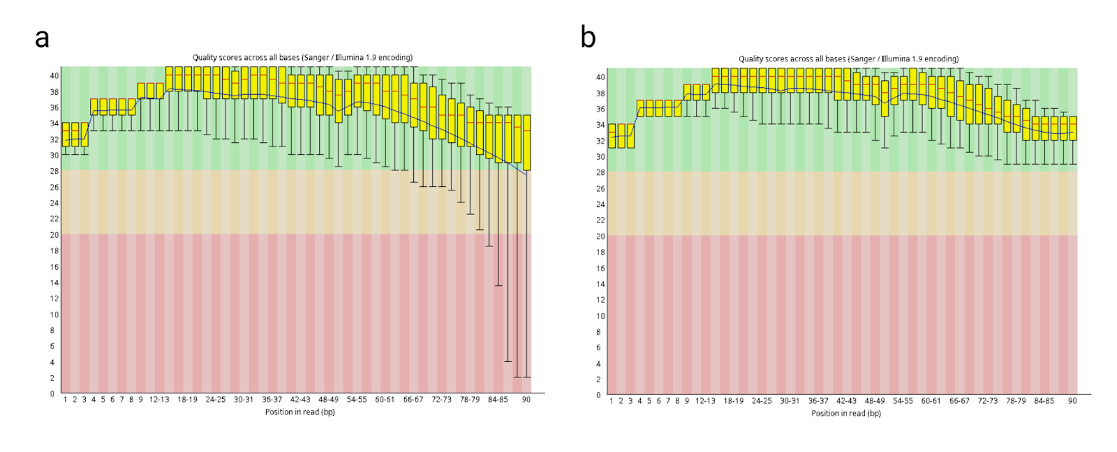
Fig. 6: Comparison of Phred quality scores of the sample SRR1278968_2 (a) before and (b) after trimming.
This confirms that we have successfully trimmed our RNA-Seq data by removing the low quality and short reads while preserving the majority of high-quality data. We can now move on to subsequent analyses.
RNA-Seq Read Mapping and Quantification
Runtime: See below for specific steps.
In this tutorial, our goal is to find genes that are differentially expressed between pathogenic and non-pathogenic forms of the human fungal pathogen C. parapsilosis. In order to assess differential expression, we first need to obtain “expression values” for genes of this yeast. In this section, we’ll show you how to calculate read counts for each gene (which are proportional to gene expression levels) using two different methods:
-
The “classical” approach: Read mapping to a reference genome with subsequent calculation of mapped reads in each gene.
-
The pseudo-mapping approach: Direct calculation of expression levels from the fastq files and reference transcripts.
There are advantages and disadvantages to each of these approaches. The main advantage of pseudo-mapping is that it’s extremely fast and requires very little RAM usage, while the classical approach is quite computationally demanding and can be relatively slow (depending on which software you use). Additionally, pseudo-mapping is just one step, while classical read-mapping involves two steps. (First read-mapping, then calculating the number of reads mapped to each gene.) Finally, read-mapping creates sam/bam files, which require a lot of hard drive space. Pseudo-mapping readily generates much smaller files with expression values.
On the other hand, a “classical” read mapping offers one important advantage over the pseudo-mapping approach: The large sam/bam read alignment files it creates allow us to perform many other valuable types of analysis on RNA-Seq data. That includes variant calling, novel transcript discovery, and calculation of species proportions when several organisms are sequenced as one sample (for example in case of host-microbe interaction studies, metatranscriptomics studies, etc.). In contrast, pseudo-mapping has far more limited applications, and is mainly used to assess gene expression levels.
In a normal RNA-Seq analysis, your choice of read-mapping method will depend on the specific research question you’re investigating. In this tutorial, we’ll show you how to perform both of these approaches.
Reference genome fetching
For both read-mapping methods, we will need a reference genome and genome annotations. Our first step is to obtain that data from a special database for Candida species called Candida Genome Database. Go go to the ref_gen directory and download both files with the following commands:
wget http://www.candidagenome.org/download/sequence/C_parapsilosis_CDC317/current/C_parapsilosis_CDC317_current_chromosomes.fasta.gz
wget http://www.candidagenome.org/download/gff/C_parapsilosis_CDC317/C_parapsilosis_CDC317_current_features.gff
gunzip C_parapsilosis_CDC317_current_chromosomes.fasta.gz
In this code, the wget commands will download the reference genome and genome annotation in gff format for C. parapsilosis. The gunzip command will uncompress the genome file. With these two files, we can perform both read mapping and pseudo-mapping.
Read mapping and counting using STAR software
First, we will perform read mapping and read calculation using STAR – a popular, versatile software package for RNA-Seq read-mapping. STAR is very fast, offers a wide variety of options and analyses, and comes with excellent user support. Another important advantage of STAR is that it can calculate the number of reads mapped to each gene during the mapping process, so we won’t need to use any additional software. For our analysis of yeast data, STAR will need just 2-3 GB of RAM.
To use STAR, let's first install it in our rnaseq environment. Run this command:
conda install star --channel conda-forge --channel bioconda --channel defaults --strict-channel-priorityTo begin read mapping, we first need to index the reference genome:
Index the reference genome: _Run time ~10 seconds on workstation, 20 seconds on mac _
To index the genome, first run the following command:
STAR --runThreadN 2 --runMode genomeGenerate --genomeDir cpar --genomeFastaFiles C_parapsilosis_CDC317_current_chromosomes.fasta --genomeSAindexNbases 10Before proceeding, let’s explore what this command is doing:
--runThreadN 2 tells STAR to use 2 cores
--runMode genomeGenerate tells STAR to perform genome indexing
--genomeFastaFiles sets the genome to be indexed (C_parapsilosis_CDC317_current_chromosomes.fasta)
--genomeDir cpar tells STAR to write the index to the cpar directory.
--genomeSAindexNbases is specific to our genome. We are setting the value to 10 (vs. the default value of 14) because the size of the C. parapsilosis genome is small.
See the STAR manual for more details on these parameters.
Convert the file format of genome annotations The final step before we can perform read mapping is to convert the original genome annotations (which are in gff format) to gtf format. This is necessary because gtf is the preferred format for STAR to count reads for downstream differential gene expression analysis. For this conversion, we'll use the gffread tool (Pertea and Pertea 2020).
First, install gffread in the environment:
conda install gffread --channel conda-forge --channel bioconda --channel defaults --strict-channel-priorityNow run gffread with this command:
gffread C_parapsilosis_CDC317_current_features.gff -T -o C_parapsilosis_CDC317_current_features.gtfRead mapping
Runtime: ~20 min on the Workstation, ~1 hour on the Mac
Now that we have indexed the reference genome and converted the original annotations to gtf format, we can proceed with the actual read mapping. First, go to the mapping directory with this command:
cd ../mapping/To run the read mapping for all samples, we will use the following script:
while read f; do
echo "STAR --runThreadN 2 --genomeDir ../ref_gen/cpar/ --sjdbGTFfile ../ref_gen/C_parapsilosis_CDC317_current_features.gtf --readFilesIn ../raw_data/trimming/${`f`}_tr_1P.fastq.gz ../raw_data/trimming/${`f`}_tr_2P.fastq.gz --readFilesCommand zcat --outFileNamePrefix ${f}_ --outSAMtype BAM SortedByCoordinate --limitBAMsortRAM 3000000000 --quantMode GeneCounts”
done`<../raw_data/sample_ids.txt`
This simple script will iterate over the file names we have written in the raw_data/sample_ids.txt file and print the STAR command for each file. Let’s explore this script in greater detail:
--runThreadN 2 tells STAR to use 2 CPU cores (change this number if you have more/fewer cores)
--genomeDir navigates STAR to the reference genome index
--sjdbGTFfile navigates to the gtf file
--readFilesIn specifies the trimmed input files for each sample
--readFilesCommand zcat is necessary to read the fastq files in a compressed format (Note: if you are using a Mac computer, change “zcat” to “gzcat”.)
--outFileNamePrefix ${f}_ specifies the prefix of the output files
--outSAMtype BAM SortedByCoordinate tells STAR to generate sorted bam files
--limitBAMsortRAM 3000000000 directs STAR to use a maximum 3 GB of RAM for bam file sorting (which is enough in our case)
--quantMode GeneCounts tells STAR to perform read calculation for each gene, generating the values that we need for differential expression analysis.
Now run this command:
bash mapping.sh > star_commands.txtThis will output all the above-mentioned commands to a file called star_commands.txt. As in our trimming step, this file can be either run as a bash command or submitted as an array job in computing clusters. Here we will use the bash command:
bash star_commands.txt
Note for Mac usersIf STAR 2.7.10a throws a “Segmentation fault” error when the mapping step starts, please install an older version of STAR.
Upon finishing the read mapping for each sample, STAR produces several output files. Their names will begin with the value we set via the --outFileNamePrefix option (i.e. with the corresponding sample name). Our main output files will be the following:
- Aligned.sortedByCoord.out.bam – a sorted read alignment file in bam format
- Log.final.out – a final concise log file of STAR mapping
- ReadsPerGene.out.tab – a file containing the read count data which will be used for differential gene expression analysis
Checking success of read mapping
To ensure our read mapping was successful, let's inspect several parameters in the Log.final.out files. Open the file SRR1278968_Log.final.out, and let's review these three parameters:
- Uniquely mapped reads %
- % of reads mapped to multiple loci
- % of reads unmapped: too short
Uniquely mapped reads % tells us what percentage of total reads were mapped uniquely to the reference genome. The higher this number is, the better. Values between 85% and 95% are considered a good mapping rate. In our case, that number is 96.80%, which is quite high.
% of reads mapped to multiple loci indicates the percentage of reads that are mapped to more than one genomic position. These are called multi-mapped reads, and it’s difficult to know their true place of origin. The multimapping rate is typically high for samples originating from genomes with highly repetitive regions, preventing the software from mapping the reads uniquely to those regions. In our case, the multimapping rate is 2.21%, which is low.
% of reads unmapped: too short indicates the percentage of reads that did not map to the reference because the alignment of that read to the genome was too short. Obviously, the lower this number is, the better. For our sample, the unmapped reads constitute only 0.98%.
So far, we have only reviewed one of many log files. To simplify this process, we can aggregate the statistics from many log files using MultiQC. In the mapping folder, run this command:
multiqc .When the analysis is finished, open the file multiqc_report.html in your browser. You should see an image like the one below (Fig. 7), which nicely illustrates our mapping statistics in a single plot:
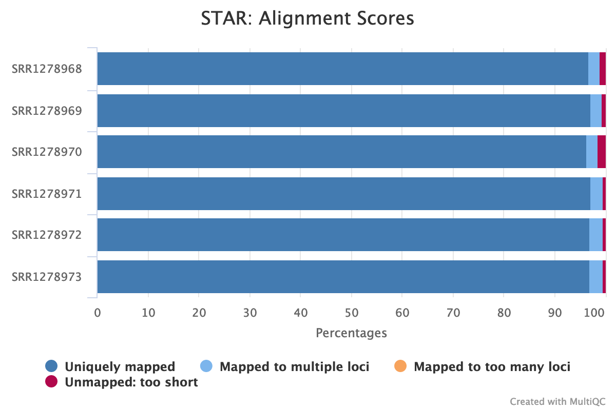
Fig. 7: An aggregated plot of STAR mapping statistics for all analyzed samples.
As we discussed above, STAR also generates ReadsPerGene.out.tab files, which contain read counts of genes (i.e. how many reads were mapped to each gene) in C. parapsilosis. Let’s review one example – the file SRR1278968_ReadsPerGene.out.tab. This file has four columns which correspond to different strandedness options:
- Column 1 – gene name
- Column 2 – counts for unstranded RNA-seq
- Column 3 – counts for forward-stranded data
- Column 4 – counts for the reverse-stranded data
We already know that our data is stranded, per the original paper by Holland et al., 2014. And in the MultiQC plot called “Gene Counts” (Fig. 8, below) we can clearly see that most reads are assigned to genes in reverse-stranded configuration:
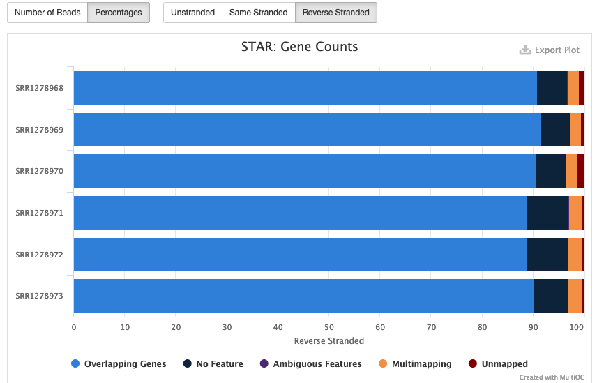
Fig. 8: Reads counts of all samples depending on strandedness configuration.
This means that our RNA-Seq data is reverse-stranded. Thus, we will need to use the data in column 4 for differential gene expression analysis. More details about RNA-Seq strandedness can be found here and here.
We have now performed read mapping for all RNA-Seq samples of C. parapsilosis using STAR mapper. The software has additionally calculated the number of reads mapping to each gene. This data will be used later to perform differential gene expression analysis.
Visualization of RNA-Seq bam files
Runtime: Depends on how long you spend investigating the data.
In this section, we will visualize the bam files we obtained during read mapping to make our analysis more intuitive and clear. We will use Integrative Genomics Viewer (Robinson et al. 2011) (IGV), which is a powerful and versatile java application for visualizing genomics data. But before our bam files can be visualized, they must first be sorted and indexed. They have already been sorted via STAR mapper, which we used for read mapping. To index them, we will use the program samtools (Li et al. 2009).
First, install samtools in the rnaseq environment using this command:
conda install samtools --channel conda-forge --channel bioconda --channel defaults --strict-channel-priorityNow let’s index one of the bam files that we have generated in the previous step. Run the following command:
samtools index SRR1278973_Aligned.sortedByCoord.out.bamNext, install and launch IGV with these commands:
conda install -c bioconda igv
igv
This will open a graphical user interface for the program. Go to Genome > Load Genomes from File > select the genome fasta file of C. parapsilosis. The chromosomes of the yeast will appear at the top of IGV. Now go to File > Load from file > select the gff annotation file of C. parapsilosis. The genome annotations will appear underneath the chromosome, showing genes and other annotated elements of the genome. We can right-click on the annotations track, and select the “Expanded” option to see all genomic features more clearly. Next, go to File > Load from file > select the indexed bam file SRR1278973_Aligned.sortedByCoord.out.bam.
When this file is selected, IGV will create two tracks – one with a coverage line plot (at the top), and a second, larger track visualizing all mapped reads. To see both of these plots, select one chromosome from the dropdown menu, then zoom in using the + sign at the top-right corner. After zooming in sufficiently, the coverage plot and the reads will appear. They should look like this:
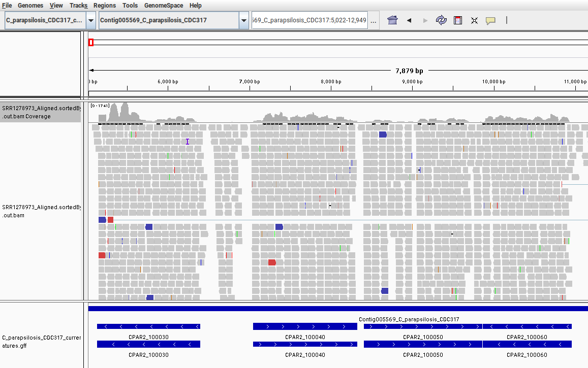
Fig. 9: Screenshot from IGV showing the mapped RNA-Seq data to the C. parapsilosis reference genome. Only a small region in the beginning of the chromosome “Contig005569” is shown.
In this image, we can see that different genes have different coverages. This means that each gene has a different number of reads mapped to it, reflecting its expression levels. In our read-counting section, we counted the number of mapped reads that fall within the range of each gene. We have now visualized these relationships with IGV.
Get to know Integrative Genome Viewer (IGV)IGV is very powerful, flexible software that can visualize and analyze many other features of mapped reads. We highly recommend spending more time with it to explore its many functions!
Read quantification using Salmon software
Runtime: See below for indexing and pseudo-mapping steps.
In this section, we will explore an alternative approach to calculating read counts in each gene from our RNA-Seq samples. We will use Salmon software, which performs a so-called pseudo-mapping (or pseudo-alignment) analysis to directly quantify the read counts and expression levels of genes from fastq files and reference transcripts. Salmon and similar software such as kallisto (Bray et al. 2016), are extremely fast, require very little RAM, and do not produce the “classical” sam/bam alignment files, which require a lot of storage space.
To perform this analysis, we will need to complete three steps:
- Obtain a fasta file of genes/transcripts of C. parapsilosis
- Index that fasta file
- Perform pseudo-mapping
We’ll use gffread to perform the first step, and Salmon to perform the second and third steps.
First let's install both software packages. We recommend installing them in a new, separate conda environment. The following command both creates a new salmon_env environment and installs Salmon and gffread software to it:
conda create -n salmon_env salmon gffread  --channel conda-forge --channel bioconda  --channel defaults --strict-channel-priority
conda activate salmon_env
Obtain a fasta file of genes/transcripts of C. parapsilosis
Next, let's obtain the fasta file with gene sequences for C. parapsilosis. We’ll use gffread, which extracts the gene sequences from the reference genome of C. parapsilosis based on the information of the gff file. In the ref_gen directory, run this command:
gffread -w transcripts.fasta -W -F -g C_parapsilosis_CDC317_current_chromosomes.fasta C_parapsilosis_CDC317_current_features.gffThis command creates the file transcripts.fasta, which contains the sequences of C. parapsilosis genes (based on exon information in gff files)
Now let’s create two new directories in our initial folder and go to the first one:
mkdir -p salmon/ref_gen salmon/mapping
cd salmon/ref_gen/
Index the fasta file with Salmon Runtime: 5 seconds on the Workstation, 30 seconds on the Mac
Next, we will create an index of the transcripts.fasta file called cpar_index, to which we then will perform the pseudo-mapping. Run the following commands to perform the indexing:
salmon index -t ../../ref_gen/transcripts.fasta -i cpar_indexPerform pseudo-mapping _Runtime: 4 min on the Workstation, 15 minutes on the Mac _
Once the indexing is finished, we can perform the pseudo-mapping. First, switch to the salmon/mapping directory:
cd ../mapping/Now run the following script called salmon_mapping.sh:
while read f;do
echo "salmon quant -i ../ref_gen/cpar_index/ -l A" \
"-1 ../../raw_data/trimming/${f}_tr_1P.fastq.gz" \
"-2 ../../raw_data/trimming/${f}_tr_2P.fastq.gz" \
"-p 2 --validateMappings -o quants/${f}_quant"
done`<../../raw_data/sample_ids.txt`
As in our previous trimming and read mapping steps, this script iterates over the sample names in the sample_ids.txt file, and for each sample prints out a salmon command for pseudo-mapping. Let’s review this command in more detail:
-i directs Salmon to the cpar_index
-l A tells Salmon to automatically detect strandedness of data
-1 and -2 supply the reads to Salmon
-p 2 tells Salmon to use 2 cores
--validateMappings increases sensitivity of Salmon
-o specifies the name of the output folders.
To generate these Salmon commands, run this command:
bash salmon_mapping.sh > salmon_commands.txt
Finally, use this command to run Salmon:
bash salmon_commands.txtUpon completing this task, Salmon will produce several output files. The file salmon_quant.log will contain information about mapping rates. To aggregate the result of all samples, we can use MultiQC. Run MultiQC with this command:
multiqc .Now open the generated report in your browser. The general statistics and mapping rates should look like this:
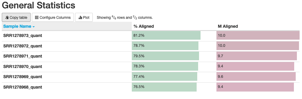
Fig. 10: General statistics and mapping rates of Salmon runs.
In this plot, we can see that our “% Aligned” data averages around 78%, which is lower than the number we found when read mapping via STAR. This is somewhat expected because Salmon “aligns” the reads only to known genes/transcripts that we supply to it, while STAR maps reads to the entire genome and can capture data originating from non-annotated genes/transcripts.
The main output file of Salmon, which contains the gene expression data, is called quant.sf. Let's open the file quants/SRR1278968_quant/quant.sf. This file has 5 columns:
- Name - gene/transcript name
- Length - gene/transcript length
- EffectiveLength - gene/transcript effective length (see here for details)
- TPM - Transcripts Per Million (TPM) expression levels (see more details about this in the following sections)
- NumReads - an estimated number of reads “mapped” to genes/transcripts
The data in our final column – NumReads – can be used for differential gene expression analysis.
To summarize, we have just performed a fast, lightweight read counting with pseudo-mapping using Salmon software. We can now move on to differential gene expression analysis.
RNA-Seq Differential Gene Expression Analysis
We have arrived at the final stage of our RNA-Seq workflow! In this step, we will perform a differential gene expression analysis of C. parapsilosis comparing its biofilm and planktonic conditions, thus revealing which biological processes are implicated in biofilm formation. But before we proceed, let's review some technical background to better understand gene expression.
What is Gene Expression
Gene expression can be viewed as the number of mRNA molecules present in the cell at a given moment in a given condition. As we’ve discussed several times in this tutorial, the read count data that we obtained in the previous section using STAR/Salmon are not the gene expression values per se, but are proportional to them.
Let’s imagine a very rough example. Consider a cell with two genes, A and B, which have the same length. At a given time, there are 10 and 50 mRNA molecules for each gene, respectively – the proportion between them is 1:5. In an RNA-Seq analysis of these genes, the absolute number of read counts can vary, depending on sequencing depth. With a low sequencing depth, our respective reads may be 300 and 1505, while a high sequencing depth may generate 5020 and 25200 reads. But in both cases, their proportion remains very close to the real proportion of mRNA molecules – 1:5 (assuming no technical biases). Knowing this, we can be confident that our analysis reflects true gene expression levels.
Note that normalization plays a critical role in RNA-Seq data analysis. There are different approaches to normalization, and the correct approach will depend on which type of comparison you’re making.
For within-sample comparisons – i.e. when comparing different genes of one sample – we need to account for both gene length (because longer genes will generate more reads) and library size (i.e. the total number of sequenced reads). The units of expression obtained after accounting for library size and then for gene length are called Read Per Kilobase Million (RPKM, which is used for single-end reads), and Fragments per Kilobase Million (FPKM, which is used for paired-end reads). Another unit of expression which accounts for both factors is called Transcripts Per Million (TPM), and it is now the most popular unit for within-sample comparisons. Learn more details about the difference between RPKM, FPKM, and TPM here.
For between-sample comparisons, gene length does not matter because we are comparing the same gene across different samples. In these cases, Trimmed Mean of M values (TMM) is one of the preferred means of normalization.
RNA-Seq data normalization is a topic of extensive research, and we have only briefly covered it here. For more details, we recommend some of these readings as a jumping-off point:
RNA-Seq Conda Profile Construction
In this tutorial, we are performing a differential gene expression analysis, which is a between-sample comparison. To find differentially expressed genes, we will use the popular Bioconductor package DESeq2 implemented in R. Then we will visualize differentially expressed genes using Microarray (MA) plots. Finally we will perform GO term enrichment analysis of up-regulated genes using two methods – an online tool at Candida Genome Database, and using the clusterProfiler Bioconductor package in R.
First, let’s install necessary software. We recommend creating a separate Conda environment called dif_exp. In your terminal, run the following commands:
conda create -n dif_exp
conda activate dif_exp
Now install the software using these commands:
conda install bioconductor-biocparallel
conda install -c bioconda bioconductor-deseq2
conda install -c bioconda bioconductor-clusterprofiler
conda install -c conda-forge r-ggpubr
Alternatively, you can install the first three software packages within R using the corresponding Bioconductor installation pages. (For example, see instructions for installing DESeq2 here.) The last package, ggpubr, can be installed within R using this command:
install.packages("ggpubr")From this point forward, we'll be using R language. We will run scripts from a terminal via the Rscript command, but you can also run them in Rstudio IDE.
To keep our mapping directory clean, let’s make a new directory called DE and go there using these commands:
mkdir DE
cd DE
In the next sections, we'll perform the differential gene expression analysis, visualize it, and conclude with GO term enrichment analysis.
Differential Gene Expression & Visualization
Runtime: 10 seconds on the Workstation, 1 minute on the Mac
First, we will perform differential gene expression analysis and visualize the obtained results. We'll use the script DE.R, which is fully contained in this recipe:
RNA-Seq Differential Gene Expression Analysis rna-seq-differential-gene-expression-analysis
Now we'll break down the recipe to better understand how our differential gene expression analysis works. The code below is repeated from the recipe above – we're just displaying it here for reference purposes. The script has five steps, which we'll explore one by one:
Step 1: Load the libraries and set the working directory
library(DESeq2)
library(ggpubr)

setwd("/path/to/mapping/")
In this step, we load the necessary software (DESeq2 and ggpubr) and set our working directory to the mapping directory, where the output files of STAR are located.
Step 2: Load the read count data from STAR
data<-NULL
for (f in c("SRR1278968_ReadsPerGene.out.tab","SRR1278969_ReadsPerGene.out.tab","SRR1278970_ReadsPerGene.out.tab",
"SRR1278971_ReadsPerGene.out.tab", "SRR1278972_ReadsPerGene.out.tab", "SRR1278973_ReadsPerGene.out.tab"))
{
file<-read.table(f,header = TRUE, sep = "\t")
data<-cbind(data,file[,4])
}

rownames(data)<-file[,1]
colnames(data)<-c("SRR1278968", "SRR1278969","SRR1278970",
"SRR1278971", "SRR1278972","SRR1278973")
data<-data[-c(1,2,3),]
Here we are loading the read count data generated by STAR into R, and making a dataframe called data. In essence, this piece of code creates an empty dataframe, and (using the for loop) iteratively populates it with the read counts from the fourth column of each ReadsPerGene.out.tab file. It then uses our sample names to assign column names to this new dataframe, and uses gene names for the rows. The final data frame looks like this:
| SRR1278968 | SRR1278969 | SRR1278970 | SRR1278971 | SRR1278972 | SRR1278973 | |
|---|---|---|---|---|---|---|
| CPAR2_600010 | 695 | 717 | 770 | 1915 | 1991 | 1958 |
| CPAR2_600020 | 1157 | 1087 | 1149 | 1340 | 1766 | 2428 |
| CPAR2_600030 | 361 | 375 | 436 | 787 | 819 | 764 |
Step 3: Run DESeq2
groups <- factor(c(rep("Plankton", 3), rep("Biofilm", 3)), levels=c("Plankton","Biofilm"))
colData <- DataFrame(condition=groups)
pre_dds <- DESeqDataSetFromMatrix(data, colData, design = ~condition)
dds <- DESeq(pre_dds)
res <- results(dds, contrast = c("condition", "Biofilm","Plankton"))
In this step, we run DESeq2. We then create a dataframe colData which contains the condition of each column in data. The first three columns (samples SRR1278968, SRR1278969, and SRR1278970) are planktonic state. The last three columns are biofilm state. The final colData is a single-column table that looks like this:
| Condition |
|---|
| Plankton |
| Plankton |
| Plankton |
| Biofilm |
| Biofilm |
| Biofilm |
Note that we also specified levels=c("Plankton","Biofilm"). Without this important specification, DESeq2 will define the reference levels in alphabetical order – i.e. it will make “Biofilm” the reference level. (What we want is the opposite – “Plankton” should be the reference.) levels=c("Plankton","Biofilm") instructs DEseq2 to give us the comparison based on the last factor, i.e. Biofilm against Plankton.
We then create a DESeq2 object from data and colData, and using the design = ~condition we state that we want to make all different comparisons based on condition – in our case, biofilm vs plankton.
The line dds <- DESeq(pre_dds) runs the DESEq2 program.
DESeq2 performs some sophisticated analyses to assess differential expression. First, it conducts its own internal normalization of read count data across all samples by calculating so-called size factors, which normalize for library size and compositional biases. Then it performs some complex statistical analysis using generalized linear models in order to calculate fold-changes and p-values for desired comparisons. (More details about DESeq2 can be found in the original DESeq2 paper.)
The last line of step 3 specifies which comparison we want to retrieve from the DESeq2. Using contrast, we state that we want the biofilm condition to be compared to the planktonic one. In other words, if we observe a gene with up-regulated expression, this gene is up-regulated in the biofilm state. This contrast option is somewhat redundant, because we have already set the comparison levels in colData when setting the order of levels. Regardless, we recommend using contrast to be on the safe side.
The results of the differential gene expression analysis are written to a variable called res. In essence, this is a dataframe with the following data:
baseMean – mean of normalized counts from all samples
log2FoldChange – log2 fold-change between tested conditions
lfcSE – standard error of log2 fold-change
stat – Wald statistics
pvalue – Wald test p-value
padj – adjusted p-value for multiple testing
In our ongoing analysis, we will consider a gene to be differentially expressed if it expression has changed more than 4 times (|log2 fold change|>2), and padj<0.01. These filters can be changed depending on how strict we want to be.
Step 4: Visualize the results
ggmaplot(res, main = "Differential expression in Biofilm vs Planktonic form",
    fdr = 0.01, fc = 4, size = 3,
    palette = c("red", "blue", "darkgray"),
    legend = "top", top = 0)
ggsave("./DE/maplot.png")


norm_data<-vst(dds)
plotPCA(norm_data,ntop=5000)
ggsave("./DE/pca.png")
In this step, we are creating high-level visualizations of our differential gene expression results. We first create an MA plot of all results using the ggmaplot command. The output is saved (using the ggsave command) as a file called maplot.png. If you open this file, it should look like this:
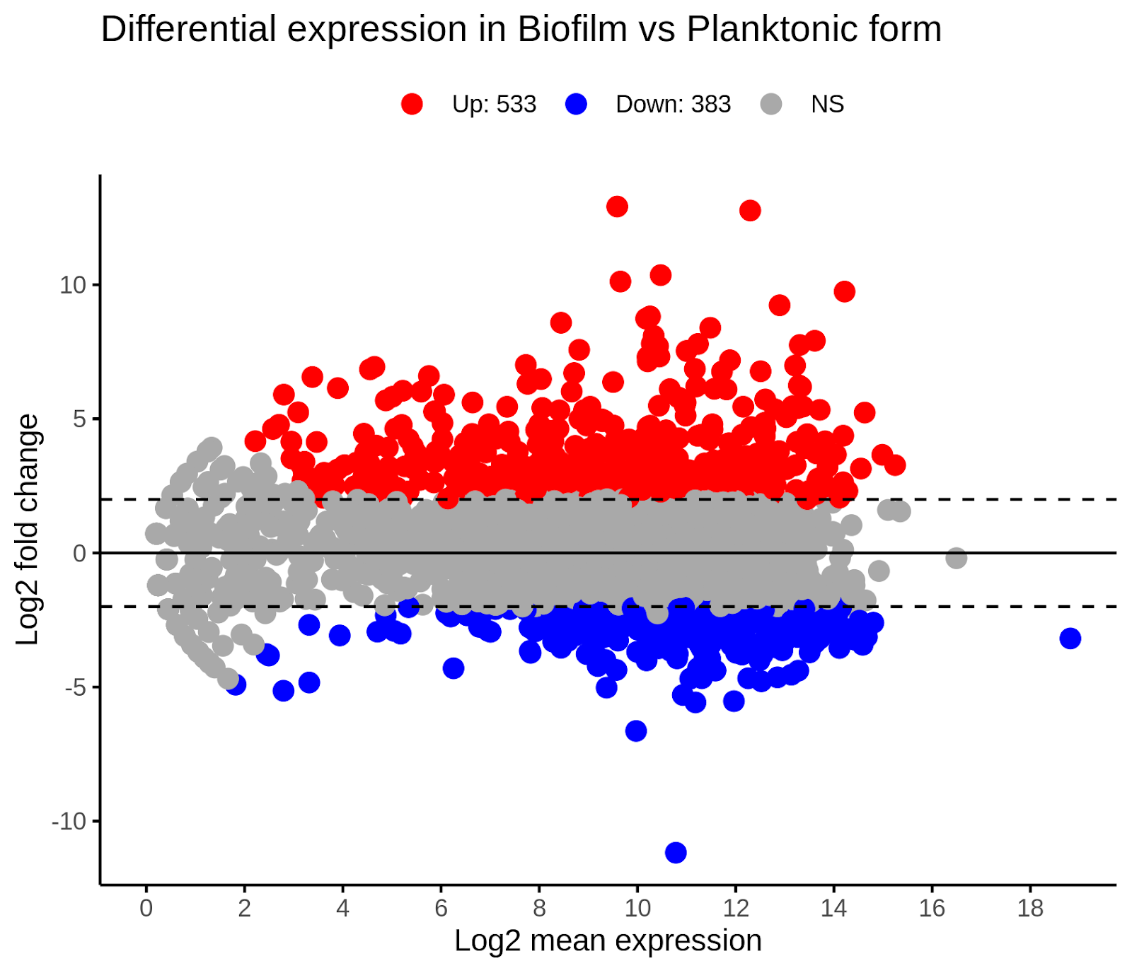
Fig. 11: MA-plot of differential gene expression analysis. Up - up-regulated genes, Down - down-regulated genes, NS - not significant.
In this image, we can see that the biofilm state contains 533 up-regulated genes and 383 down-regulated genes relative to the planktonic state.
The next command in step 4 is plotPCA, which creates a Principal Component Analysis (PCA) plot. This plot gives us an important holistic picture of the data by showing the distribution of samples in 2D space:
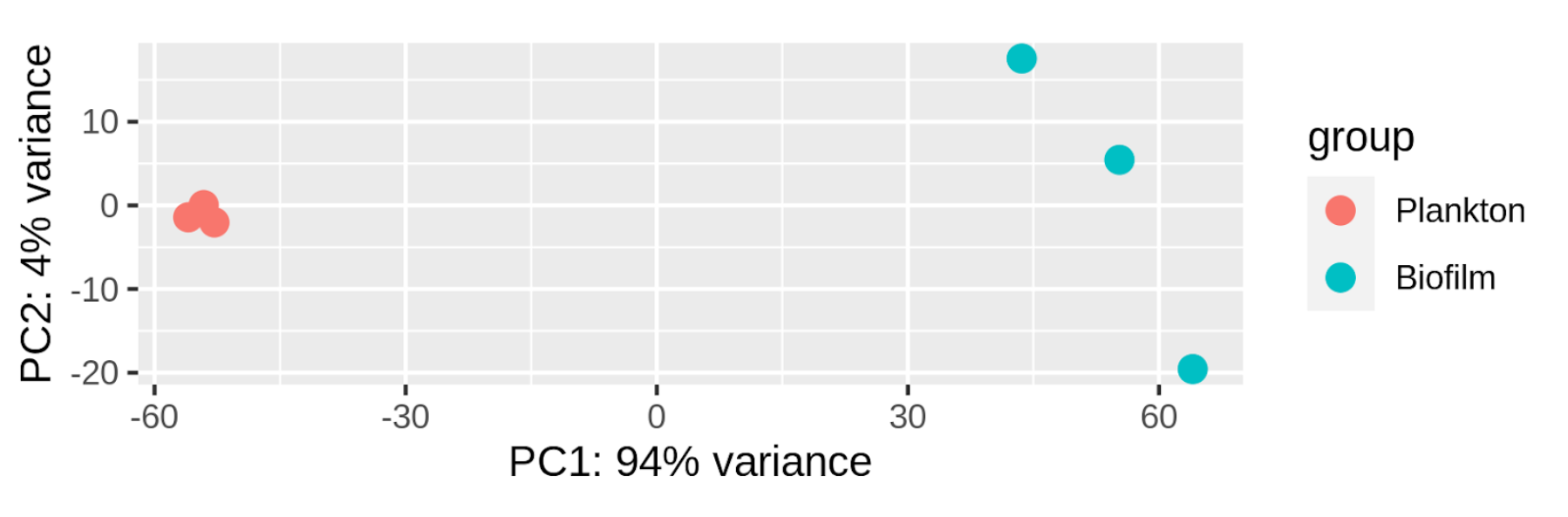
Fig. 12: PCA plot of analyzed samples. Percentages on both axes show the amount of variance explained by each axis.
From this image, we learn that A) there is a large difference in gene expression levels between planktonic and biofilm states of C. parapsilosis, and B) that there is high variability among samples of biofilm.
For more complex experimental designs, PCA plots can help detect batch effects. In this case, however, we don't know whether the library preparations of samples in both conditions were done at once or in batches. This makes it impossible to judge how much variation between the two states is true biological variation and how much is due to batch effects.
Step 5: Export the up-regulated genes
upreg_in_biofilm<-row.names(res[!is.na(res$padj) & res$log2FoldChange > 2 & res$padj<0.01,])

write.table(upreg_in_biofilm, file="./DE/up_regulated_genes.txt", sep = "\t", quote = FALSE, col.names = F, row.names = F )
In this final step, we are exporting the up-regulated genes in biofilm to a separate file called up_regulated_genes.txt. This file will be used to assess the functional implications of these genes in biofilm formation of C. parapsilosis using GO term enrichment analysis.
To summarize this section, we have just performed a differential gene expression analysis of C. parapsilosis in two states using the popular software DESeq2. We visualized the obtained results and exported the up-regulated genes to a file which will be used in downstream analysis to discern the functional roles of these genes.
Go Term Enrichment Analysis
Gene Ontology (GO) term enrichment is a quick way to gain insights into the functional implications of gene sets of interest. In this tutorial, we are interested in whether the up-regulated genes we’ve detected in biofilm are implicated in certain biological processes. We will perform the GO enrichment analysis in two different ways – first via manual search, then via automated script.
Manual GO Enrichment
First, we’ll use an online GO Term Finder tool available through the Candida Genome Database. To begin, visit the database’s GO Term Finder page. Select the species Candida parapsilosis. Under Upload a file of Gene/ORF names, upload the file up_regulated_genes.txt. Now click Search.
When this analysis is finished (in ~1 minute), the site will bring us to a new page. At the bottom of this page, you will see a table with your GO term enrichment analysis results. It will look like this:
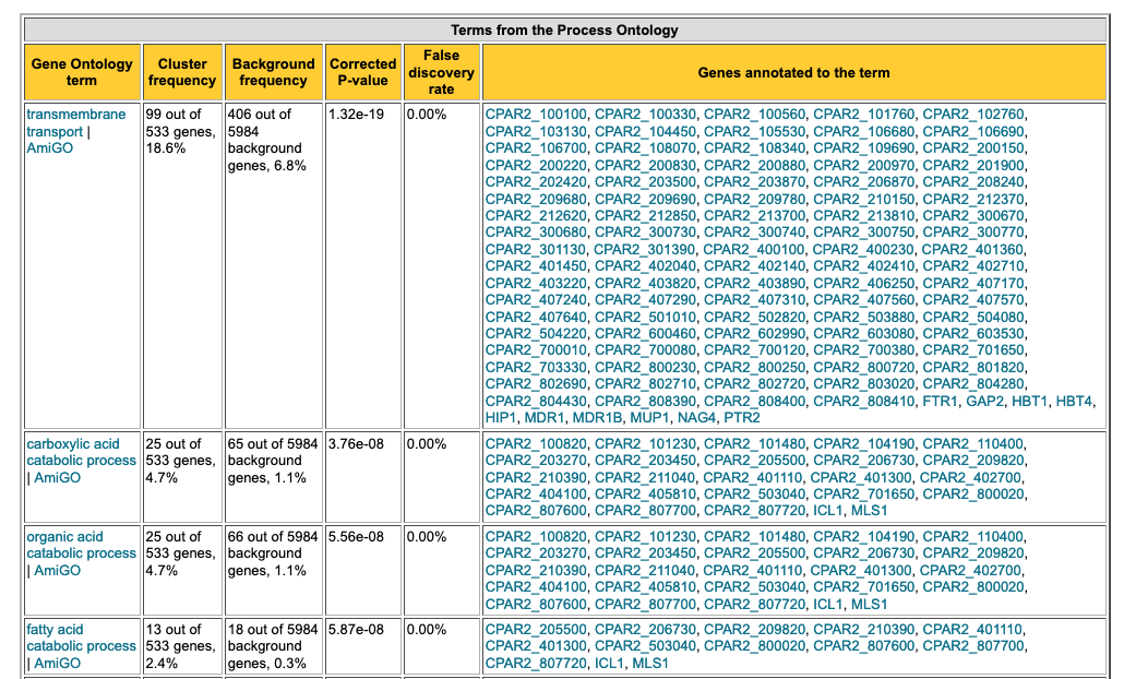
Fig. 13: Example of GO term enrichment analysis table generated by GO Term Finder at Candida Genome Database.
In this table, you can see that the up-regulated genes in biofilm are implicated in various biological processes, including transmembrane transport, catabolism, lipid oxidation, iron transport, etc. These biological processes are thus likely triggered in the process of biofilm formation in this yeast. Knowing this can help us design more specific experiments to investigate the mechanism of biofilm formation in greater detail (for example, disrupting certain genes/pathways to find novel targets for potential antifungal drugs).
Programmatic GO Enrichment
Now imagine that we need to perform hundreds of GO term enrichment analyses. This would obviously be quite tedious using the above manual method. Instead, let’s automate the entire process using the Bioconductor package clusterProfiler and perform the enrichment programmatically in R.
Note that clusterProfiler can readily perform GO term enrichment analysis for model organisms (such as human data) using the list of genes of interest. This is because it is internally connected to GO term databases of model organisms. C. parapsilosis is not a model organism, meaning that clusterProfiler (like other generic tools and websites) does not readily support the analysis of its data. However, clusterProfiler can perform enrichment analysis for any species if we supply it with the necessary GO term data. To make clusterProfiler work for C. parapsilosis, we first need to obtain and prepare the GO term data for this yeast, and then perform the enrichment analysis.
For this step, we will use a script called GO.R, which you can find in the following recipe:
Programmatic GO Term Enrichment Analysis using clusterProfiler programmatic-go-term-enrichment-analysis-using-clusterprofiler
Let's explore how this recipe works. Below, we'll display its code for reference purposes, but don't worry – it's all fully contained in the recipe above. The script has five steps, which we'll explore one by one.
Step 1: Load the libraries and set the working directory
library(clusterProfiler)
library(GO.db)

setwd("/path/to/mapping/DE/")
In this step, we load the necessary software (clusterProfiler and GO.db) and set our working directory to DE.
Step 2: Obtain GO terms of C. parapsilosis
all_go_tems<-as.data.frame(GOTERM)
all_go_tems<-all_go_tems[!(all_go_tems$go_id %in% c("GO:0003674","GO:0008150","GO:0005575")),]
BP_terms<-all_go_tems$go_id[all_go_tems$Ontology=="BP"]

cpar_go<-read.table("path/to/cpar_go.txt")
BP_universe<-cpar_go[cpar_go$V1 %in% BP_terms,]
In this step, we will retrieve all possible GO IDs for Biological Process terms (and remove some very general GO IDs). The last two lines load the GO IDs of_ C. parapsilosis_ (via the file cpar_go.txt, which can be retrieved from the Candida Genome Database, or downloaded here), and select only GO IDs of Biological Process. The final BP_universe dataframe should look like this:
| V1 | V2 | V3 |
|---|---|---|
| GO:0055085 | CPAR2_303940 | P |
| GO:0015867 | CPAR2_303940 | P |
| GO:0015886 | CPAR2_303940 | P |
Step 3: Associate GO ID with description
goterms <- Term(GOTERM)
a<-as.data.frame(goterms)
go_names<-cbind(row.names(a),a)
In this step, we construct a dataframe called go_names which contains GO IDs and their descriptions:
| row.names(a) | goterms | |
|---|---|---|
| GO:0000001 | GO:0000001 | mitochondrion inheritance |
| GO:0000002 | GO:0000002 | mitochondrial genome maintenance |
| GO:0000003 | GO:0000003 | reproduction |
Step 4: Load up-regulated genes and run clusterProfiler's enriched
upreg_in_biofilm <- read.table("./up_regulated_genes.txt",header = FALSE)
upreg_in_biofilm <- as.character(upreg_in_biofilm$V1)


ego<-enricher(upreg_in_biofilm, universe = as.character(BP_universe$V2), TERM2GENE = BP_universe,TERM2NAME = go_names)
Now that we have two dataframes (BP_universe and go_names), we can perform the GO enrichment analysis. First, we load the files with up-regulated genes obtained in the differential expression analysis. Then we supply these genes to the clusterProfiler function enricher. This function performs a hypergeometric test to find significant GO term enrichments of the supplied list of genes in the GO term universe. The results will be written to the ego variable.
Step 5: Visualize GO terms
dotplot(ego,showCategory = 15)
ggsave("./up_reg_go_terms.png")
Finally, we use the dotplot function of clusterProfiler to visualize the results of GO term enrichment. This saves an output file called up_reg_go_terms.png. If you open the file, it will look like this:
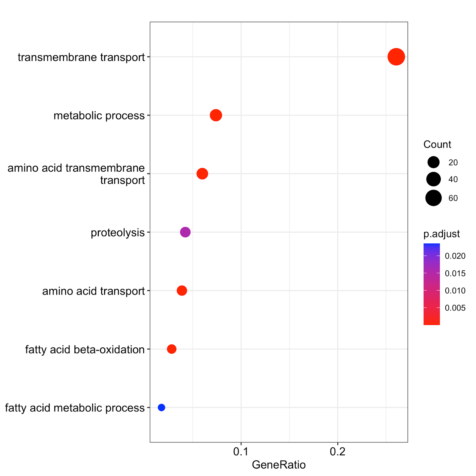
Fig. 14: The results of GO term enrichment analysis obtained using clusterProfiler. Count refers to the total number of genes assigned to GO categories. GeneRatio corresponds to the ratio between the number of input genes assigned to a given GO category and Counts. Only significant (padj<0.05) enrichments are shown. Adjustment of p-values is done by Benjamini-Hochberg procedure.
These results are similar to our manual GO term enrichment analysis via the Candida Genome Database – but we obtained them in an automated and programmatic manner. This approach works for any non-model organism for which the GO terms are available. ClusterProfiler is versatile software with many parameters and visualization options, so we encourage you to play around with it and explore its rich functionality.
To summarize this section, we have just successfully performed functional GO term enrichment analysis and visualization of the up-regulated genes of C. parapsilosis in the biofilm state. We then automated this step using clusterProfiler software.
Background: What Is RNA-Seq?
RNA plays a key role in most cellular processes. To understand cellular behavior, we thus need to study the identity, function, and abundance of RNA molecules (i.e. transcripts).
And while this has long been a scientific goal, recent advances in massively parallel nucleic acid sequencing (also known as Next-Generation Sequencing, or NGS) have transformed the way we study biology. The study of RNA is no exception: NGS-based RNA sequencing technology – aka RNA-Seq – has created unprecedented opportunities to investigate RNA transcripts in a genome-wide manner,
RNA-Seq is now the principal method used in transcriptomics studies, largely superseding other technologies such as gene expression microarrays. It is a versatile and relatively cheap technology that allows us to study transcriptomes in a qualitative and quantitative manner without requiring prior knowledge of the transcripts.
RNA-Seq has a wide range of scientific applications. That includes the study of gene expression, the identification of novel transcripts/isoforms, the study of RNA structure, and the analysis of RNA-RNA/protein interactions, among many others. Broadly speaking, RNA-Seq consists of two major steps: designing a study and sequencing your samples, then running downstream bioinformatics analysis. But beyond that, specifics can vary greatly.
In this tutorial, we will perform a differential gene expression analysis. This is a fairly common, standardized procedure, with steps you can follow in any similar real-life project. But please note that it’s just one example of a very flexible, powerful analytical approach. RNA-Seq is capable of much more, and your specific analysis may look very different.
In the next section, we’ll explore experimental principles and guidelines for designing an RNA-Seq-based analysis of differential gene expression.
RNA-Seq Experimental Design
Transcriptomes are highly dynamic, sensitive systems that can be easily influenced by external factors. That means good experimental design is essential to any RNA-Seq project. By “experimental design,” we mean the type of study (treatment-vs-control, time-course, observational study, etc.) as well as how it is planned and performed from a logical and technical perspective. Without this careful planning and execution, your experiment can yield spurious and misleading results.
For example, in a poorly-planned RNA-Seq treatment-vs-control experiment, the “control” samples might be exposed to hidden/unnoticed treatments (i.e. non-standard culturing medium, different temperature, etc). On the other hand, a well-planned design can still be poorly executed – e.g. if the treatment and control samples are prepared in different institutions by different people. In both scenarios, the results will suffer from so-called confounders and/or batch effects, leading to incorrect conclusions. In other words, experimental planning and execution are equally important.
This is why it is critical to carefully plan and execute your RNA-Seq projects, especially when tackling complex research questions with multiple conditions, comparisons, time-points, etc. We strongly recommend you invest serious time and resources in this step before performing the actual experiments and sequencing. You may also want to consult with more experienced professionals if your team is new to RNA-Seq. These measures can save you time and money in the long run – and most importantly, they’ll strengthen your scientific outcomes.
In the following sections, we’ll review some key considerations around experimental design in your RNA-Seq analysis.
Descriptive vs Comparative Designs
When planning an RNA-Seq gene expression study, you’ll choose between a descriptive and a comparative design.
In a descriptive study, you’re simply identifying which genes are expressed in a sample and (typically) observing their expression levels under normal conditions. This kind of study is mainly used for species that have not been previously characterized on a genomic/transcriptomic level.
In a comparative study, you’re analyzing a sample’s gene expression levels across multiple conditions (e.g. cancer vs healthy tissue, normal vs stress conditions, time-series, etc.). This reveals how gene expression is influenced by a certain condition.
Generally speaking, comparative study design is more involved and complex than descriptive study design. This is because it presents greater opportunity for errors (such as confounding and batch effects) which can only be prevented via careful experimental planning and execution. In this tutorial, we’re performing a differential gene expression analysis. This is a classic comparative study, since we are comparing gene expression across multiple conditions.
Hypothesis-Generating vs. Hypothesis-Testing Studies
RNA-Seq-based gene expression studies can be formally classified into two types: hypothesis-generating and hypothesis-testing experiments.
In a hypothesis-generating study, the researchers do not begin with a specific and concrete question of interest about the investigated biological system. Instead, they simply aim to generate as much data as possible and hope to discover interesting patterns and connections. Hypothesis-generating experiments are typically large-scale projects that involve many samples, variables, conditions, etc. Ideally, they produce interesting results that other researchers can forge into specific, testable hypotheses.
In contrast, a hypothesis-testing experiment is performed to test a specific question of interest – e.g. what happens to genes of a certain pathway when the cells are exposed to a given stressor. Normally, this type of experiment is more compact, as it may test only one condition. The drawback, however, is that it is quite hard to integrate data from these experiments with data from other projects due to batch/confounding effects.
Some studies contain both hypothesis-generating and hypothesis-testing phases. This means researchers first generate a large volume of data, then test a specific hypothesis that emerges from it. This was the structure of Holland et al, 2014, which yielded the data we will analyze today.
Different Types of RNA Selection
A living cell contains many types of RNA, such as mRNAs, microRNAs, lncRNAs, tRNAs, rRNAs, etc. Depending on the research question at hand, you may wish to sequence all of them or just a subset. This choice will inform your RNA selection protocols.
To take just one example, it is known that the vast majority of RNA in bacterial or yeast cells is represented by ribosomal RNA. In essence, rRNA is just several very highly expressed transcripts. Sequencing that kind of sample will yield very little data about other important transcripts, such as mRNAs that encode for proteins. It would thus be recommended to experimentally deplete rRNAs before performing the sequencing (for bacteria) or select only mRNAs, e.g. by using poly-A tails selection (for yeasts).
In this tutorial, we’re working with data from a study by Holland et al, 2014. Neither the study itself nor the SRA database identifies which type of RNA selection was used to obtain the original data. Fortunately, this will not impact our RNA-Seq data analysis.
Stranded vs Non-Stranded Library Preparation Protocols
RNA molecules are transcribed from either the positive (+) or negative (-) strand of a double-stranded DNA molecule. When you’re working with an RNA transcript, it is virtually always helpful to know which DNA strand it originated from.
Early methods for extracting RNA from samples and preparing so-called sequencing libraries were not able to preserve this information, leaving researchers in the dark about the origin of their transcripts. This was particularly troublesome because many species contain overlapping genes which are located at the same DNA position but on different strands. For example, yeasts encode thousands of so-called antisense transcripts – RNA transcripts originating from the opposite strand of protein-coding genes. Hence, it is crucial to know the strand information to discriminate between the protein-coding genes and antisense RNAs.
Fortunately, today we have several strand-specific library preparation protocols available. These protocols can keep track of the strand of origin, and their use is strongly recommended when executing an experimental design. The data we’re analyzing in this tutorial was generated using strand-specific library preparation protocols.
Sequencing Depth & Read Length
After RNA extraction, RNA selection, and library preparation, it is time to decide how much sequencing data is needed from each sample for a robust downstream analysis. In other words, we need to determine our sequencing depth.
This question is rarely trivial and typically depends on the species to be analyzed. There are several studies that systematically address this issue in the realm of human genetic research – and while not ideal, these studies can serve as a rough benchmark for other species. In one of these studies, researchers found that sequencing more than 10 million reads for the human genome does not substantially add power to detect differentially expressed genes. On the other hand, the Encode guidelines for sequencing depth in differential gene expression analysis recommend 30 million reads per sample. Fortunately, the cost of generating sequencing data has dropped significantly in recent years thanks to the development of ultra-high throughput sequencing machines like Illumina NovaSeq. Thus, aiming for 30-40 million reads will place us on the safe side for a reasonable budget.
To determine the read length for our RNA-Seq data (i.e. the length of short stretches of cDNA molecules which are actually sequenced), we also need to consider the internal characteristics of our analyzed species. In the case of the human genome, it is recommended to get paired-end reads with a length of at least 50 base pairs (bp). For a yeast, single-end data of 50 bp should be sufficient.
Please note that the sequencing depth and read length discussed here are adequate only for differential gene expression analysis. These parameters may be inappropriate for other types of RNA-Seq analysis, such as novel transcript discovery, isoform usage, etc.
Replicates
In differential gene expression analysis, our main goal is to identify genes which changed their expression to a statistically significant degree due to an investigated condition. Thus, to perform our statistical analysis, it is absolutely crucial to have replicates. While technical replicates (i.e. the same sample divided into several parts) are advisable but not strictly necessary, it is necessary to obtain true biological replicates of the sample for robust statistical analysis.
For example, if we’re comparing gene expression in cancerous vs normal tissue, a biological replicate would be samples from different individuals. Similarly, in experiments with yeast or bacteria, biological replicates would be independently-cultured samples of the same species. The minimum number of biological replicates in a differential gene expression analysis is two (with three being highly advisable).
Replication and sequencing depth are interconnected parameters. To maintain your budget, you may need to strike a balance between adding more replicates to the study and performing deeper sequencing. Liu et al. (2014) evaluated the impact of both factors and found that, in the case of human transcriptomic data, increasing the sequencing depth over 10 million reads has diminishing incremental effects for the power of detection of differentially expressed genes. Increasing the number of biological replicates, on the other hand, significantly enhances the power of detection. Thus, for differential gene expression analysis a greater emphasis should be placed on obtaining more biological replicates.
Replicates (like the rest of your experimental setup) should be prepared together by the same technicians and in the same environments in order to avoid batch effects.
Summary
In this tutorial, we used an RNA-Seq data analysis to identify differentially expressed genes. Specifically, we found genes that are implicated in the process of biofilm formation in one of the major human fungal pathogens – C. parapsilosis. We also identified biological processes that are up-regulated during this pathogen’s plankton-biofilm transition.
RNA-Seq is a very powerful and versatile Next-Generation Sequencing technology. And while it requires some bioinformatics skills and background knowledge, we believe anyone can learn this approach with a little practice. We hope this tutorial makes differential gene expression analysis with RNA-Seq more clear, intuitive, and accessible for everyone. If there are ways we can improve it, please let us know! We’d love to hear your feedback.
References
- Abrams, Z. B., T. S. Johnson, K. Huang, P. R. O. Payne, and K. Coombes. 2019. “A Protocol to Evaluate RNA Sequencing Normalization Methods.” BMC Bioinformatics 20 (Suppl 24).
<https://doi.org/10.1186/s12859-019-3247-x>. - Bolger, A. M., M. Lohse, and B. Usadel. 2014. “Trimmomatic: A Flexible Trimmer for Illumina Sequence Data.” Bioinformatics 30 (15).
<https://doi.org/10.1093/bioinformatics/btu170>. - Bray, N. L., H. Pimentel, P. Melsted, and L. Pachter. 2016. “Near-Optimal Probabilistic RNA-Seq Quantification.” Nature Biotechnology 34 (5).
<https://doi.org/10.1038/nbt.3519>. - Conesa, A., P. Madrigal, S. Tarazona, D. Gomez-Cabrero, A. Cervera, A. McPherson, M. W. Szcześniak, et al. 2016. “A Survey of Best Practices for RNA-Seq Data Analysis.” Genome Biology 17 (January).
<https://doi.org/10.1186/s13059-016-0881-8>. - Dobin, A., C. A. Davis, F. Schlesinger, J. Drenkow, C. Zaleski, S. Jha, P. Batut, M. Chaisson, and T. R. Gingeras. 2013. “STAR: Ultrafast Universal RNA-Seq Aligner.” Bioinformatics 29 (1).
<https://doi.org/10.1093/bioinformatics/bts635>. - Evans, C., J. Hardin, and D. M. Stoebel. 2018. “Selecting between-Sample RNA-Seq Normalization Methods from the Perspective of Their Assumptions.” Briefings in Bioinformatics 19 (5).
<https://doi.org/10.1093/bib/bbx008>. - Ewels, P., M. Magnusson, S. Lundin, and M. Käller. 2016. “MultiQC: Summarize Analysis Results for Multiple Tools and Samples in a Single Report.” Bioinformatics 32 (19).
<https://doi.org/10.1093/bioinformatics/btw354>. - Holland, L. M., M. S. Schröder, S. A. Turner, H. Taff, D. Andes, Z. Grózer, A. Gácser, et al. 2014. “Comparative Phenotypic Analysis of the Major Fungal Pathogens Candida Parapsilosis and Candida Albicans.” PLoS Pathogens 10 (9).
<https://doi.org/10.1371/journal.ppat.1004365>. - Horn, D. L., D. Neofytos, E. J. Anaissie, J. A. Fishman, W. J. Steinbach, A. J. Olyaei, K. A. Marr, M. A. Pfaller, C. H. Chang, and K. M. Webster. 2009. “Epidemiology and Outcomes of Candidemia in 2019 Patients: Data from the Prospective Antifungal Therapy Alliance Registry.” Clinical Infectious Diseases: An Official Publication of the Infectious Diseases Society of America 48 (12).
<https://doi.org/10.1086/599039>. - Li, H., B. Handsaker, A. Wysoker, T. Fennell, J. Ruan, N. Homer, G. Marth, G. Abecasis, and R. Durbin. 2009. “The Sequence Alignment/Map Format and SAMtools.” Bioinformatics 25 (16).
<https://doi.org/10.1093/bioinformatics/btp352>. - Liu, Y., J. Zhou, and K. P. White. 2014. “RNA-Seq Differential Expression Studies: More Sequence or More Replication?” Bioinformatics 30 (3).
<https://doi.org/10.1093/bioinformatics/btt688>. - Love, M. I., W. Huber, and S. Anders. 2014. “Moderated Estimation of Fold Change and Dispersion for RNA-Seq Data with DESeq2.” Genome Biology 15 (12).
<https://doi.org/10.1186/s13059-014-0550-8>. - Patro, R., G. Duggal, M. I. Love, R. A. Irizarry, and C. Kingsford. 2017. “Salmon Provides Fast and Bias-Aware Quantification of Transcript Expression.” Nature Methods 14 (4).
<https://doi.org/10.1038/nmeth.4197>. - Pertea, G., and M. Pertea. 2020. “GFF Utilities: GffRead and GffCompare.” F1000Research 9 (April).
<https://doi.org/10.12688/f1000research.23297.2>. - Robinson, James T., Helga Thorvaldsdóttir, Wendy Winckler, Mitchell Guttman, Eric S. Lander, Gad Getz, and Jill P. Mesirov. 2011. “Integrative Genomics Viewer.” Nature Biotechnology 29 (1): 24.
- Skrzypek, M. S., J. Binkley, G. Binkley, S. R. Miyasato, M. Simison, and G. Sherlock. 2017. “The Candida Genome Database (CGD): Incorporation of Assembly 22, Systematic Identifiers and Visualization of High Throughput Sequencing Data.” Nucleic Acids Research 45 (D1).
<https://doi.org/10.1093/nar/gkw924>. - Wang, Z., M. Gerstein, and M. Snyder. 2009. “RNA-Seq: A Revolutionary Tool for Transcriptomics.” Nature Reviews. Genetics 10 (1).
<https://doi.org/10.1038/nrg2484>. - Yu, G., L. G. Wang, Y. Han, and Q. Y. He. 2012. “clusterProfiler: An R Package for Comparing Biological Themes among Gene Clusters.” Omics: A Journal of Integrative Biology 16 (5).
<https://doi.org/10.1089/omi.2011.0118>. - Zhao, Shanrong, Zhan Ye, and Robert Stanton. 2020. “Misuse of RPKM or TPM Normalization When Comparing across Samples and Sequencing Protocols.” RNA 26 (8): 903–9.
Updated 5 months ago