ATAC-Seq Tutorial (From Fastqs to Graphs)
Go to ai.tinybio.cloud/chat to chat with a life sciences focused ChatGPT.
This end-to-end tutorial will guide you through every step of ATAC-seq data analysis. We’ll show you how to set up your computing environment, fetch the raw sequencing data, perform read mapping, peak calling, and differential accessibility analysis, and finally visualize and interpret the results.
All you need is a reasonably modern desktop/laptop computer with a Linux/Unix-like operating system and some basic knowledge of bash and R scripting.
This tutorial primarily focuses on the bioinformatics portion of the ATAC-Seq Analysis. The background and overview can be found here. For highlights of the tutorial, see the below:
ATAC-Seq Data analysis:
In this section, we’ll guide you through every step of the ATAC-seq analysis pipeline. Each subsection contains step-by-step instructions, approximate run times, code samples, and real scripts you can use.
Before you proceed, make sure you’ve used Conda to build an environment with all the necessary software. (See Create a Computing Environment for details.) If you haven’t activated your Conda environment yet, do so now by executing this command in a terminal:
conda activate atacseqHardware Requirements
We tested this tutorial on two different computers: a workstation with Intel Core i7-8700K CPU, 3.70 GHz, and 64 GB of RAM running Open-Suse Leap 15.3 (which we’ll call “workstation”), and a 2017 MacBook Pro 2.3 GHz Dual-Core Intel Core i5 with 8 GB of RAM, running macOS Monterey 12.4 (which we’ll call “Mac”).
Given our software choices and the relatively small size of the yeast genome, all analyses will require less than 8 GB of RAM. This real-world, end-to-end ATAC-seq analysis can thus be performed even on standard consumer laptops (although with significant run-times for certain processes; see the steps below).
The entire analysis requires ~65Gb of hard drive space. Certain large files can be removed during the analysis to further reduce storage space requirements.
File System
To keep your output data tidy and organized, we suggest creating these folders in any convenient directory:
- raw_data
- raw_data/trimming
- ref_gen
- mapping
To create these folders, just run this command:
mkdir -p ./ref_gen/ ./mapping ./raw_data/trimmingThese folders will contain our entire analysis. Other folders (subdirectories) will be created on-the-go during this tutorial, but we don’t need them to begin.
Data Fetching
Run time: Depends on internet connection speed. For 50 Mbps, this step takes ~7 minutes.
We will obtain our ATAC-seq data using SRA Explorer – an online tool for efficiently searching and downloading raw sequencing data. First, go to the SRA Explorer site. In the search field, paste the following SRA project ID:
PRJNA576599Select all six samples and add them to your collection. Now go to saved datasets and download the “Bash script for downloading FastQ files”.
Optional: If the IBM Aspera proprietary client is available on your device, we recommend downloading the data with Aspera commands. This can significantly increase your download speeds.
Now locate the downloaded file sra_explorer_fastq_download.sh in the raw_data folder. Go to that folder with this command:
cd raw_data/By default, SRA Explorer commands rename the downloaded files. In our case, this is not necessary. To prevent the renaming, run this command:
sed "s/ATAC.*rep.*_//g" sra_explorer_fastq_download.sh > renamed_sra_explorer.shThe sed command above will simply remove the unnecessary text from the file names. Specifically, it deletes any text beginning with “ATAC” and ending with “rep…_”. After renaming, simply run the command below to download the sequencing data.
bash renamed_sra_explorer.shWhen the data is downloaded, create a text file containing the file names of the samples:
ls SRR*gz | cut -f 1 -d "_" | sort | uniq > sample_ids.txtFor some downstream steps such as trimming and mapping, we will iterate over this file (i.e. read each of its lines) and run analyses for each sample.
Data Quality Control
Run time: ~3 minutes on workstation with 2 cores, and ~60 minutes on Mac with 2 cores
Now we need to perform quality control of the raw sequencing data to ensure that only high quality reads are used moving forward. For this step, we’ll use FastQC, which analyzes the fastq files (the data format of the raw sequencing data) and reports important statistics and parameters of the data. To run FastQC (v. 0.11.9), first create a directory called fastqc_initial, and then run the fastqc command:
mkdir ./fastqc_initial
fastqc -t 2 *fastq.gz -o ./fastqc_initial
In this command, the term fastqc.gz means that FastQC will analyze all files in the current directory ending with fastq.gz and store the results in the fastqc_initial directory. The parameter -t 2 instructs FastQC to use two cores of the computer.
Because FastQC reports the results for each fastq file separately, we now have 12 html quality reports to review. Rather than inspect these one-by-one (which would be tedious), we’ll use the MultiQC tool* (v. 1.12) to aggregate them. First, navigate to the fastqc_initial folder, then run MultiQC:
cd ./fastqc_initial/
multiqc .
MultiQC will scan the current directory and collect the output files of FastQC, generating a single, beautiful html report of all our samples. (Note that MultiQC can handle output from numerous software types – e.g. mappers, trimmers, etc. – to create informative, interactive, publication-ready reports.) To inspect the aggregated report, open the multiqc_report.html in your web browser. You can use either of these commands:
firefox multiqc_report.htmlopen multiqc_report.htmlYour MultiQC report should look like this:
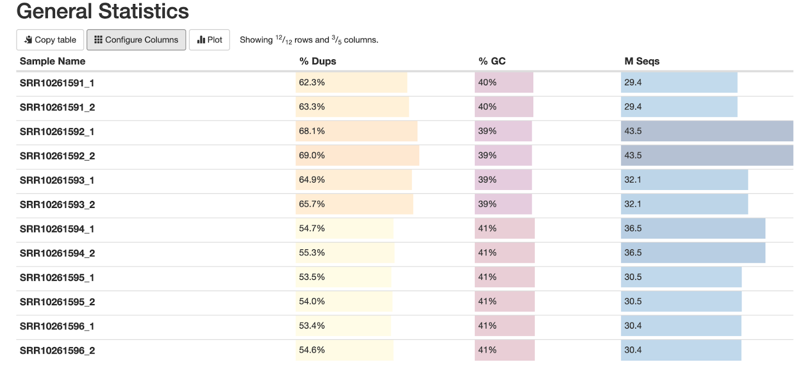
Fig. 3: The general statistics of the analyzed fastq samples, showing the sample names, duplication percentages, GC content percentages, and the number of sequencing reads.
This plot shows the overview of our data and its main parameters. Let's review some of its features:
First, notice that our percentage of duplicated reads ("% Dups") is relatively high. This is to be expected in ATAC-seq data, as the sequenced regions are generally short. This can generate identical reads – especially in cases like ours, where data is high-coverage. These numbers also indicate PCR duplicates, which are technical artifacts and will be removed in later steps of our workflow.
Second, our GC content of ~39-40% is expected for S. cerevisiae and S. uvarum, and is a good signal that the data is not contaminated. And finally, the last column indicates the numbers of sequencing reads. As mentioned above, each sample has ~30 million reads per each direction (i.e. 60 million paired-end reads).
Let's move on to another part of our MultQC report: the Phred score plot. Phred score is an important metric of sequencing read quality. It indicates the reliability of each sequenced base (learn more here), with values between 30 and 40 considered good scores:
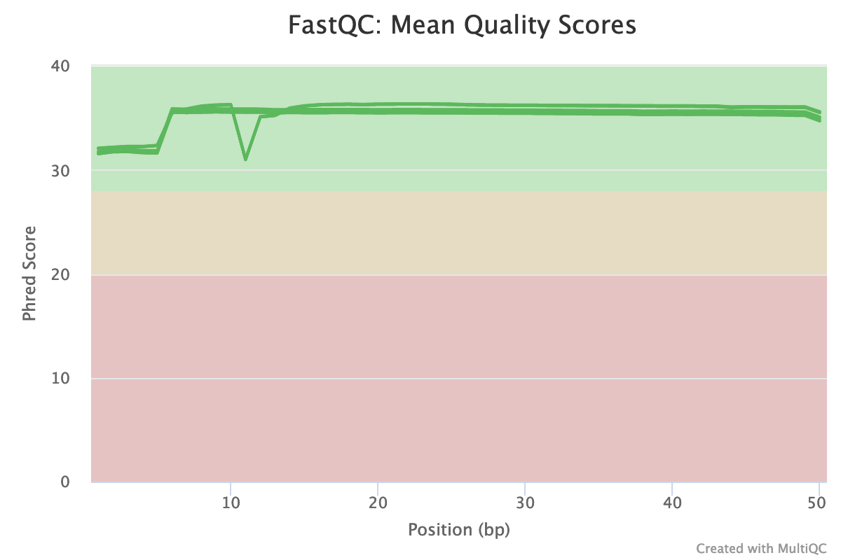
Fig. 4: Mean Phred-quality scores of each sample
The plot above illustrates the quality scores of each base position in all samples (each line corresponds to a sample). Although there is a dip at position 11 in some samples, the overall quality of the ATAC-seq data is very high. That means our data does not need any correction for this metric.
Finally, let's review this chart of our adapter content:
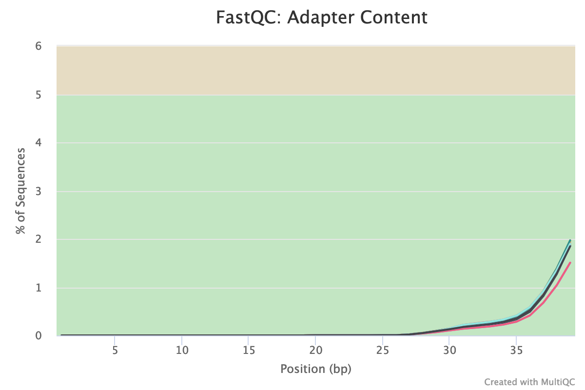
Fig. 5: Presence of Nextera adapters sequences in all studies samples.
The presence of adapter sequences (which are inserted into the DNA during the experimental sample preparation) is an important parameter of our sequencing data. Adapter sequences can interfere with downstream analyses (for example by reducing the read-mapping rate), and thus should be removed from the data if present. As you can see above, our samples contain trace amounts of Nextera transposase adapter sequence, starting from the middle of the reads. These should be trimmed away in order to improve the quality of the data. (We'll tackle that in our next section.)
In summary, our quality control analysis using FastQC and MultiQC has revealed that the ATAC-seq data has high overall quality, but contains trace amounts of adapter sequences which should be removed before further analysis.
Trimming
Run time: ~50 minutes on workstation with 2 cores, ~30 hours on Mac with 2 cores.
We will use the popular read-trimming software Trimmomatic (v. 0.39) to perform this step. For paired-end sequencing data, Trimmomatic expects two input files (one per sequencing direction), and outputs four different files: forward-paired reads, forward-unpaired reads, reverse-paired reads, and reverse-unpaired reads. The unpaired reads are generated when one read of a pair does not survive the trimming, but the other one does. For the downstream analysis, only paired reads are typically used.
To begin the read trimming process, navigate to the raw_data/trimming folder:
cd ./trimmingThe following simple bash script trimming.sh will generate Trimmomatic commands for each sample:
while read sample_id; do
    echo trimmomatic PE -threads 2 \
    ../${sample_id}_1.fastq.gz ../${sample_id}_2.fastq.gz \
        ${sample_id}_tr_1P.fastq.gz ${sample_id}_tr_1U.fastq.gz\ ${sample_id}_tr_2P.fastq.gz
        ${sample_id}_tr_2U.fastq.gz \
ILLUMINACLIP:~/miniconda2/envs/atacseq/share/trimmomatic-0.39-2/adapters/NexteraPE-PE.fa:2:30:10 MINLEN:30
done <../sample_ids.txt
Before we continue, let's break down how this script works. It iterates over the sample names contained in the sample_ids.txt file we created earlier, generating a Trimmomatic command for each sample. In the output files (which end with tr_1P.fastq.gz), “P” stands for “paired”, and “U” stands for unpaired. The ILLUMINACLIP parameter navigates to the fasta file with Nextera adapters (which should be located in the Conda/Miniconda environment). The parameters 2:30:10 tell Trimmomatic to cut the adapters allowing a maximum of 2 mismatches, a score of 30 for paired reads, and score of 10 for single reads (see the Trimmomatic manual for more details about this score). And the MINLEN option tells Trimmomatic to drop reads shorter than 30 base pairs.
To generate the Trimmomatic commands, run:
bash trimming.sh > trimming_commands.txtThis command creates a trimming_commands.txt file containing all commands for trimming. These can either be run as a bash command or submitted as an array job in slurm/sge/other cluster schedulers. For this tutorial, we will use this command:
bash trimming_commands.txt 1>trimming_output 2>trimming_errorThis will run the trimming commands and redirect standard output and standard error to corresponding files. After the trimming is finished, we will create a new folder fastqc_trimming and run FastQC and MultiQC to check the trimmed data. Let's use these commands:
mkdir fastqc_trimming
fastqc -t 2 *P.fastq.gz -o fastqc_trimming/
multiqc .
MultiQC will now create another html report – but this time, it will also contain statistics around our Trimmomatic output:
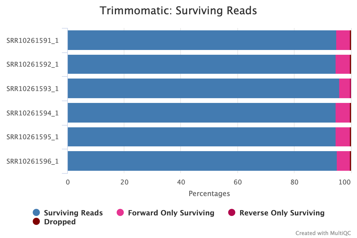
Fig. 6: Summary statistics of trimming results reported by MultiQC.
This report shows that only a small percentage of reads were dropped due to trimming, suggesting that our trimming has gently removed the few unnecessary reads. It also shows that our trimming of adapters was successful and there are no samples found with adapter contamination.
In summary, we have just successfully trimmed our ATAC-seq data, removing the unnecessary adapter sequences and remaining short reads while preserving the majority of high-quality data for downstream analysis.
Mapping & Related Analyses
Run time: See below for each type of analysis
We have arrived at the longest and most computationally demanding step of this workflow: sequencing read mapping to corresponding reference genomes, which will generate the open chromatin profiles of samples originating from the ATAC-seq experiment. This step consists of two parts – reference genome fetching/indexing and read mapping itself (with some auxiliary analyses).
Reference genome fetching and indexing
Run time: ~20 seconds on workstation, ~10 min on Mac
In order to map the sequencing data to the reference genomes, our reference genomes must first be obtained and indexed. The reference genome and genome annotation of S. cerevisiae are available in the Ensembl database (PMID: 34791404). To download them, go to the mapping/ref_gen directory and run the following commands:
wget http://ftp.ensembl.org/pub/release-106/fasta/saccharomyces_cerevisiae/dna/Saccharomyces_cerevisiae.R64-1-1.dna.toplevel.fa.gz
wget http://ftp.ensembl.org/pub/release-106/gtf/saccharomyces_cerevisiae/Saccharomyces_cerevisiae.R64-1-1.106.gtf.gz
gunzip Saccharomyces_cerevisiae.R64-1-1.*
The first two wget commands will download the genome and annotations, respectively, and the gunzip command will uncompress them. The genome annotation (i.e. gtf file) is only necessary for data visualization in later steps.
One peculiarity of the S. cerevisiae genome is that it contains two clusters of ribosomal (rRNA) genes on chromosome XII (region 450915-469179 and 489349-490611). This can result in problematic alignments during the mapping step, especially in ATAC-seq data analysis. To avoid this, we will mask these regions of chromosome XII using bedtools v. 2.30.0 (Quinlan 2014).
Note that this masking step is specific to S. cerevisiae, and may not be necessary for other organisms.
First, create a bed file named mask_rRNA.bed containing these regions:
XII    450915    469179
XII    489349    490611
Then run:
bedtools maskfasta -fi Saccharomyces_cerevisiae.R64-1-1.dna.toplevel.fa -bed mask_rRNA.bed -fo S_cerevisiae_masked_rRNA.fastaThis will create the masked genome file S_cerevisiae_masked_rRNA.fasta.
Next, we need to obtain the reference genome of S. uvarum. It can be downloaded with these commands:
wget http://www.saccharomycessensustricto.org/current/Sbay/Sbay.ultrascaf
wget http://www.saccharomycessensustricto.org/current/Sbay/Sbay.unplaced
cat Sbay.ultrascaf Sbay.unplaced > S_uvarum.fasta
The last command simply concatenates the two fasta files of S. uvarum into a single genome file.
Because the samples contain data from the S. cerevisiae parent and the hybrid S. cerevisiae x S. uvarum, we will need to artificially create the genome of the hybrid by concatenating the genomes of the two species in one file:
cat S_cerevisiae_masked_rRNA.fasta S_uvarum.fasta > hybrid.fastaThe fastq data of S. cerevisiae will be mapped to the parental genome, while the data from the hybrid will be mapped to the hybrid genome. This will separate the reads between the two organisms and further select only the data from S. cerevisiae.
Once the final genome files S_cerevisiae_masked_rRNA.fasta and hybrid.fasta are ready, they can be indexed for further read mapping.
The read mapping (and thus indexing) will be performed using the popular short-read mapping software BWA v. 0.7.17-r1188 with MEM algorithm. To index the genomes with BWA, create a file indexing.sh with the following commands:
bwa index -p SC  S_cerevisiae_masked_rRNA.fasta
bwa index -p hybrid hybrid.fasta
Then run:
bash indexing.shNow that we have fetched and indexed our reference genomes, we can map our fastq data to them.
Read mapping and related analyses
Run time: ~90 minutes on workstation, ~ 70 hours on Mac.
Now we will map the reads of the trimmed fastq files to the corresponding reference genomes. We will also sort and index our alignment files, calculate read mapping statistics, mark the duplicated reads, and subset the S. cerevisiae data from the hybrid.
For simplicity, the entire analysis is divided into two parts:
- Read mapping, sorting, indexing, and calculation of mapping statistics
- Subsetting of S. cerevisiae from hybrid, marking duplicated reads, and indexing and calculating statistics of the remaining data.
For the first part, the following script will be used:
while read sample; do
    if [ ${sample} == SRR10261591 ] || [ ${sample} == SRR10261592 ] || [ ${sample} == SRR10261593 ]; then
   	 ref_gen=SC
    else
   	 ref_gen=hybrid
    fi

    echo "bwa mem -t 2 ./ref_gen/${ref_gen} ../raw_data/trimming/${sample}_tr_1P.fastq.gz ../raw_data/trimming/${sample}_tr_2P.fastq.gz | samtools sort -@2 -o ${sample}.bam -" \
   	 "&& samtools index ${sample}.bam" \
   	 "&& samtools flagstat ${sample}.bam > ${sample}_map_stats.txt"
done<../raw_data/sample_ids.txt
This script will iterate over the sample names in sample_ids.txt file. In the if statement, the script decides to which reference genome each sample will be mapped. If the samples are SRR10261591, SRR10261592, or SRR10261593 (i.e. the samples originating from the S. cerevisiae parent), the mapping will be done to S. cerevisiae (i.e. SC), otherwise to hybrid.
Next, this script will perform read mapping with bwa mem, which will generate the output file in a so-called sam/bam format (learn more about these formats). Then these output files will be sorted (i.e. samtools sort), indexed (i.e. samtools index), and used for calculation of mapping statistics (i.e. samtools flagstat). These three steps will be performed using samtools v. 1.6 software (Li et al. 2009). This sorting and indexing process will allow us to perform various helpful downstream analyses, such as visualization and mapping statistics calculation.
Run the script with this command:
bash map_sort_index_stat.sh > map_sort_index_stat_commands.txtThis will output all the above mentioned commands to map_sort_index_stat_commands.txt file. As in our trimming process, this file can be either run as a bash command or submitted as an array job in computing clusters. We will use the bash command:
bash map_sort_index_stat_commands.txtWhen finished, inspect the *map_stats.txt files to view the mapping statistics. You will see that over 80% of reads are mapped and properly paired for all samples, indicating a successful mapping.
Before we can proceed in peak-calling our ATAC-seq data, three auxiliary analyses need to be performed:
- First, because the hybrid samples contain data from both Saccharomyces species, we need to select the S. cerevisiae data in those samples.
- Second, in ATAC-seq analysis it is generally recommended to remove mitochondrial data before the peak calling analysis. This is because the mitochondrial genome (mtDNA) does not have chromatin and so is “naked,” meaning a high proportion of ATAC-seq data can originate from mtDNA. This can lead to false peaks. In other words, we will select only non-mtDNA S. cerevisiae data from all samples for further analysis.
- Third, as described above in the PCR Amplification section, ATAC-seq data can contain a high proportion of PCR-duplicated reads. These are technical artifacts from experimental procedures and need to be removed/masked for the downstream analysis.
To perform these three analyses, we’ll use the script subset_markdupl_index_stat.sh:
while read sample; do
    echo "samtools view -bh ${sample}.bam I II III IV V VI VII VIII IX X XI XII XIII XIV XV XVI > ${sample}_SC_subset.bam" \
   	 "&& picard MarkDuplicates I=${sample}_SC_subset.bam O=${sample}_SC_subset_dedup.bam M=${sample}_markdup_metrics.txt" \
   	 "&& samtools index ${sample}_SC_subset_dedup.bam"    \
   	 "&& samtools flagstat ${sample}_SC_subset_dedup.bam > ${sample}_SC_subset_dedup_map_stats.txt"
done<../raw_data/sample_ids.txt
As in the previous step, this script will iterate over sample names. The term samtools view selects non-mtDNA chromosomes of S. cerevisiae (chromosome names are denoted with Roman numerals). The term picard MarkDuplicates will tag duplicated reads using Picard MarkDuplicated v. 2.27.3 software. And finally, samtools index and samtools flagstat will respectively index and calculate mapping statistics of the output files.
To generate these commands, run:
bash subset_markdupl_index_stat.sh > subset_markdupl_index_stat_commands.txtThen run:
bash subset_markdupl_index_stat_commands.txtWhen finished, inspect the *_SC_subset_dedup_map_stats.txt files (i.e mapping statistics after subsetting and deduplication). For S. cerevisiae samples, you will notice that after subsetting, the number of mapped reads remains largely unchanged. This indicates slight mitochondrial contamination. For the hybrid data, after subsetting there are still more than 20 million properly paired mapped reads for S. cerevisiae, which is more than enough for further peak calling analysis (see our previous section Data Analysis: A Quick Overview).
Peak calling
Run time: ~20 minutes on workstation, ~10 hours on Mac.
Now that we’ve obtained high-quality and high-coverage deduplicated bam files for S. cerevisiae and the hybrid, we can finally perform ATAC-seq peak calling. Peak calling identifies genomic regions which are enriched in aligned reads (to a statistically significant extent) compared to background levels. In the context of ATAC-seq, peaks will ideally correspond to the “naked” nucleosome-free DNA regions attacked by the Tn5 transposase. For this step, we will use MACS2 v. 2.2.7.1 software, which was originally designed for ChIP-seq data, but also works for ATAC-seq.
The small script below will generate commands to run MACS2 for all samples:
while read sample; do
    echo "macs2 callpeak -t ${sample}_SC_subset_dedup.bam -f BAMPE -n ${sample}_peak -g 12000000 --keep-dup all"
done<../raw_data/sample_ids.txt
Let’s explore some important parameters here. First, -f BAMPE tells MACS2 that the data is paired-end and directs the software to analyze only properly-paired reads, which are abundant in our sample. Second, the option –keep-dup all tells MACS2 that PCR duplicates were handled by other software (picard MarkDuplicates in our case). And third, the option -g 12000000 denotes the effective genome size of S. cerevisiae (~12Mb).
Run the script with the following command to generate the MACS2 commands:
bash call_peaks.sh > call_peaks_commands.txtThen run:
bash call_peaks_commands.txtUpon completion, MACS2 generates several outputs for each sample:
- peaks.narrowPeak file: A BED6+4 format file which contains the peak locations together with peak summit, p-value, and q-value
- peaks.xls file: A tabular file which contains information about called peaks. Additional information includes pileup and fold enrichment
- summits.bed file: Peak summit locations for every peak.
We have now performed an ATAC-seq analysis and obtained the open chromatin peaks (i.e. open chromatin profiles) of S. cerevisiae in its parental and hybrid state. In the next step, we will answer our initial question of whether and to what extent S. cerevisiae changes its chromatin accessibility profiles upon hybridization. To do this, we will need to perform quality control on the obtained peaks and compare them across the two conditions (parent vs hybrid). But first, we will visualize the data generated so far in this tutorial.
Alignment & Peak Data Visualization
Run time: Depends on how long you spend investigating the data.
Our analyses to this point have yielded an array of abstract (and somewhat cryptic) results, including alignment bam files, peak files in bed format, summit files, etc. To properly integrate and interpret these results, we need data visualization. For this step, we’ll use Integrative Genomics Viewer (IGV) v. 2.4.9. IGV is a powerful and intuitive Java program that makes NGS data clear, compelling, and tangible.
Open IGV by typing igv in your terminal:
igvThis will open a graphical user interface for the program. Now go to Genome > Load Genomes for File > select the genome fasta file of S. cerevisiae. The chromosomes of the yeast will appear at the top of IGV. Then go to File > Load from file > select the gtf annotation file of S. cerevisiae. The genome annotations will appear underneath the chromosome, showing genes and other annotated elements of the genome. Next, go to File > Load from file > select one of the bam files (for example SRR10261591_SC_subset_dedup.bam).
IGV will now create two tracks for this file – one with a coverage line plot (at the top), and a second, larger track visualizing all mapped reads. To see both of them, select one chromosome from the dropdown menu, then zoom in using the + sign at the top-right corner. After zooming in sufficiently, the coverage plot and the reads will appear. The peaks of ATAC-seq should already be visible based on the coverage plot. As expected, these peaks appear in intergenic regions (i.e. between genes), where the regulatory nucleosome-free regions are located.
To visualize the peaks found by MACS2, go to File > Load from file > select SRR10261591_peak_peaks.narrowPeak file and in the same way select SRR10261591_peak_summits.bed. After loading both files, IGV will show the peaks’ regions and their summits on the corresponding tracks (tracks in IGV can be dragged and rearranged). It should look like this:
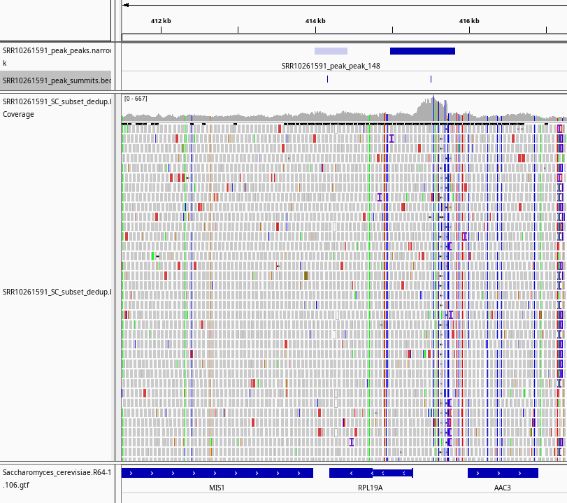
Fig. 7: Screenshot from IGV showing the integrated data for SRR10261591 sample. From the top downward, the tracks are: peaks identified by MACS2, peak summits, coverage line plot based on the bam file, aligned ATAC-seq reads, and genomic annotations of S. cerevisiae.
In this plot, you can see an intergenic ATAC-seq peak (top row, dark blue) and its summit which clearly coincides with the coverage plot of the bam file. This peak likely regulates the expression of both genes AAC3 and RPL19A, harboring some regulatory elements such as TF binding sites or promoter regions.
Again, IGV is powerful software that will integrate and clarify your results. It can visualize bam files, genome and genome annotation files, peak files, and more. IGV is a feature-reach software, and we recommend spending more time with it to explore its many functionalities.
Analysis of chromatin accessibility profile
Run time: ~5 min on workstation, ~2 hours on Mac
Now that the open chromatin states of the yeast in both conditions have been identified with MACS2, we can compare the two profiles. We will use an R Bioconductor package DiffBind v. 3.4.11 for this step.
For an effortless installation of DiffBind and its dependencies, we recommend creating a new Conda environment and installing DiffBind there as follows:
conda create -n diffbind
conda activate diffbind
conda install -c bioconda bioconductor-diffbind
The rest of this tutorial will use R language. The scripts for DiffBind analysis will be run from a terminal using the Rscript command, but you can also run them via Rstudio IDE.
To keep the mapping directory tidy, make a new directory called diffbind and go to it:
mkdir diffbind
cd diffbind
Quality control of peaks
First, it is necessary to perform the quality control of the open chromatin profiles among biological replicates in both conditions of S. cerevisiae to see whether there are any outlier samples which might bias the downstream analysis.
We’ll use the script diffbind_qc.R. Run the script from Rstudio or from the terminal with this command:
Rscript diffbind_qc.RHere is the full script:
Let's explore what's happening in the script above. First, it loads the DiffBind library, then loads the previously created peak.xls files into DiffBind. Then it performs quality control analyses among replicates of each condition, creating Venn diagrams showing how many peaks are in common across replicates:
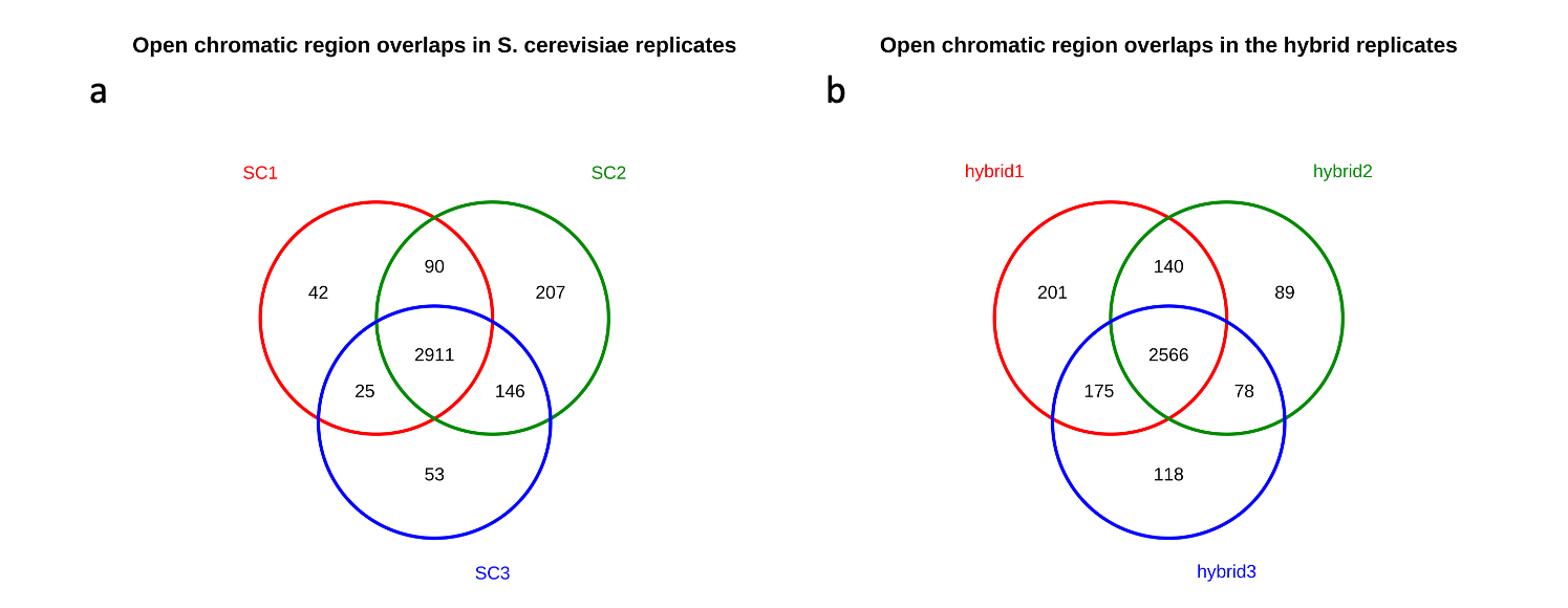
Fig. 8: Quality control analysis of open chromatin peaks between the replicates in both conditions of S. cerevisiae. (a) Overlap between the peaks in parental samples (“SC” stands for S. cerevisiae); (b) Overlap between the peaks in hybrid samples
As you can see in Fig. 8a and 8b (for parental and hybrid respectively), the vast majority of peaks are present between all replicates in both conditions. This indicates a high concordance between biological replicates in this experiment. For example, in the case of the parent, there are 2911 peaks which are in common between all replicates, while there are only 42 peaks which are specific to the replicate 1 (i.e. SC1).
DiffBind also created a heatmap plot of Pearson correlations based on previously obtained alignment bam files by calculating the number of reads in each peak across all samples:
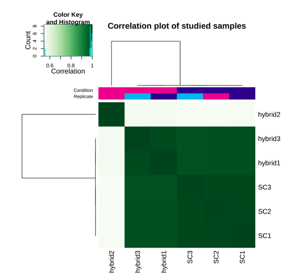
Fig. 9: Heatmap of Pearson correlations between the studies samples.
In the heatmap above, you can see that the second replicate of the hybrid represents an outlier. We will thus remove it from further analysis.
In summary, DiffBind has revealed a high overall concordance between replicates of both conditions. It also identified one outlier sample in the hybrid.
Occupancy and differential chromatin accessibility analysis
Having performed quality control between replicates of both conditions, it is now possible to compare the open chromatin profiles of S. cerevisiae between parent and hybrid. We will also use DiffBind for this step.
First, the so-called occupancy analysis will qualitatively assess how many open chromatin regions are in common between the two conditions – i.e. it will find the consensus peakset between the conditions. Second, we will perform the so-called differential accessibility analysis – the quantitative analysis showing which peaks within the consensus peakset are differentially more/less accessible due to a condition (in this case being a hybrid).
Note: To assess differential accessibility, the DiffBind package relies on DESeq2 software. DESeq2 was originally designed for differential gene expression analysis, but works well for other NGS applications such as ATAC-seq and ChIP-seq.
To run both analyses, we will use the script occupancy_and_diff_accessibility.R. You can run this script from Rstudio or from the terminal with this command:
Rscript occupancy_and_diff_accessibility.R. As in our previous quality control analysis, the script first loads the peakset and alignment files to DiffBind. (Note that we've discarded replicate 2 from this analysis because it was an outlier.) DiffBind then performs the occupancy analysis, generating a Venn diagram showing the overlap between the peaksets of the two conditions – i.e. the consensus peakset. In other words, it reveals the peaks present in both conditions:
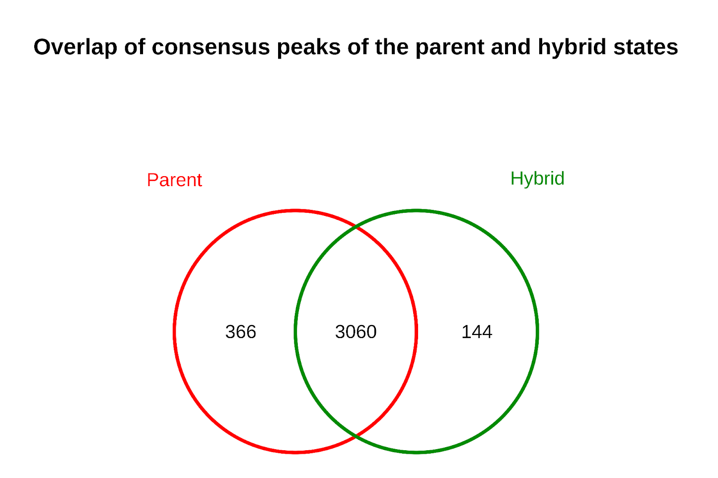
Fig. 10: Occupancy analysis and identification of the consensus peaks (n=3060) between the two conditions of S. cerevisiae.
Surprisingly, the majority of peaks are in common between S. cerevisiae in the parental and hybrid state. This indicates that chromatin accessibility profiles are largely preserved during the transition to hybrid state.
DiffBind also performs the differential accessibility analysis (sometimes called the affinity analysis), identifying differentially accessible peaks between the parent and hybrid from the consensus peakset. The output of this analysis is a table with the consensus peaks, their coordinates and chromosomes, accessibility values for both conditions, fold-change of these values, and statistical significance of the fold-change. To obtain biologically relevant results, we apply a fold-change filter of more or less than 1.0, as well as a False Discovery Rate (FDR) < 0.05. The resulting table is exported to the diffbind directory (file diff_regions_hybrid_vs_parent.txt).
In our analysis, DiffBind finds only one peak out of more than 3000 consensus peaks which is differentially open in the hybrid state compared to the parent. This strongly supports the hypothesis that open chromatin profiles (and thus gene regulation) are largely preserved in S. cerevisiae upon formation of a hybrid organism. (For scientific implications of this result, see the original paper by Hovhannisyan et al, 2020.)
Background:What is ATAC-seq
Over the past decade, advances in Next-Generation Sequencing (NGS) have disrupted life sciences. NGS has opened new horizons in the study of living systems, including their genomes, transcriptomes, chromatin states, and beyond. In recent years, NGS has been used to study gene expression regulation based on chromatin accessibility profiles in a genome-wide manner. The most powerful tool to emerge in this field is the Assay for Transposase-Accessible Chromatin using sequencing – aka, ATAC-seq.
Experimentally, ATAC-seq uses a bioengineered hyperactive transposase (Tn5) which selectively integrates its adapter sequences into regions of accessible chromatin. These regions presumably contain genomic elements regulating active transcription of downstream genes, such as enhancers, promoters, transcription factor binding sites, etc. (see Fig. 1a.) After adapter transposition, the captured regions can be amplified and sequenced.
Due to its versatility, simplicity, and sensitivity, ATAC-seq has largely superseded other similar techniques such as DNase-seq or MNase-seq (see Fig. 1b, or the original paper by Buenrostro et al, 2015, for additional technical details). In recent years, ATAC-seq protocols have been coupled to microfluidic techniques allowing open chromatin profiling on a single-cell resolution.

Fig. 1: The experimental principle of ATAC-seq. **(a)**The principle of integration of adapter sequences by Tn5 transposase into genomic loci of open chromatin regions; (b) Experimental advantages of ATAC-seq over FAIRE-seq and DNase-seq. Adapted from Buenrostro et al. 2015.
Experimental Design
Proper experimental design is essential for success in any ATAC-seq study. Like RNA-seq and other methods which characterize highly dynamic biological systems, ATAC-seq experiments and subsequent results can be influenced by various technical biases and batch effects. Even with highly sophisticated data analysis methods, it might not be possible to rescue a project that has serious flaws in the experimental design (for example, when the biological conditions are confounded with technical batch effects and biases).
It is thus critical to invest the time and resources needed to carefully plan your ATAC-seq experimental design – especially in the case of complex research questions involving multiple conditions, comparisons, time-points, etc. In this section, we’ll review some high-level design considerations.
Descriptive vs. Comparative Studies
ATAC-seq experimental design can be formally divided into two categories: descriptive and comparative:
In descriptive experiments, researchers aim to characterize the open-chromatin states of certain samples at a given condition. These results are descriptive, in the sense that they describe the number and location of open regions within the genome.
Comparative studies, on the other hand, aim to study the dynamics of chromatin states of certain samples across more than one condition (healthy vs. disease, normal vs. stress, time-series, etc). Designing a comparative study is typically more complex than designing a descriptive study.
Replicates
Biolocal (rather than technical) replicates are advisable for any NGS study to ensure that the obtained results are reproducible and real. ATAC-seq is no exception. In descriptive studies, the use of replicates is strongly recommended. And in comparative studies, it’s absolutely critical for robust statistical analysis.
At a bare minimum, two biological replicates are needed for ATAC-seq. Fewer than this will prevent you from obtaining statistically sound results. Ideally, replicates should be prepared together by the same technicians and in the same environments in order to avoid batch effects.
Sequencing Depth
“Sequencing depth” refers to the total number of sequenced reads per sample, and it must surpass a certain minimum to support robust analysis. This threshold will vary depending on the genome size, the expected number of open chromatin regions, and the type of analysis being performed. At present, however, there is no universally recognized benchmark for the optimal sequencing depth in ATAC-seq experiments (unlike, for example, in case of RNA-seq).
Nevertheless, some trustworthy guidelines exist. In the case of open chromatin detection and differential accessibility analysis for studying mammalian samples, Buenrostro et al. (2015) (the original authors of ATAC-seq) and the ENCODE project guidelines recommend having more than 50 million paired-end, non-duplicated, non-mitochondrial, uniquely mapped reads per sample. For transcription factor (TF) footprinting analysis using ATAC-seq, that number is significantly higher at 200 million recommended reads per sample (see Yan, F., Powell, D.R., Curtis, D.J. et al.)
Number of replicates and sequencing depth are the two main factors influencing the final results of an ATAC-seq project. As a rule, these two parameters constitute the largest portion of the budget for the experiments – and in many cases, budget constraints force researchers to find a tradeoff between them. If the main aim of the study is to reliably find differentially open chromatin regions, then a greater emphasis should be placed on the number of replicates (although not neglecting the recommendations of sequencing depth mentioned above). In contrast, if the aim is to perform a TF footprinting, sequencing depth should be prioritized.
Sequencing Configuration
It is highly recommended to perform paired-end read sequencing for an ATAC-seq analysis – and the longer the read length, the better. This is for several reasons:
First, paired-end reads are naturally better aligned than single-end reads since they contain twice as much information. (This is especially important when analyzing genomes with many repetitive regions.) Poor alignment in these regions can result in false-positive calls of less accessible regions.
Second, researchers are typically interested in identifying both ends of DNA fragments that originate from open-chromatin regions, since the ends indicate where transposition has occurred. This is possible only with paired-end data. (Algorithmic methods for inferring both ends of fragments from single-end data tend to be inaccurate.)
Third, paired-end reads allow us to identify true PCR duplicates more accurately and hence remove them from the analysis.
PCR Amplification
It is recommended to use as few PCR cycles as possible during library amplification. This will reduce the introduction of PCR duplicates into the ATAC-seq reads, which can interfere with the true biological signal of interest.
Create a Computing Environment
Our ATAC-seq data analysis will involve many pieces of interlinking software, all of which have their own versions and dependencies. To ensure this software meshes appropriately, we need a package management system. This tutorial will use Conda – an open-source package and environment management system that runs on every major operating system.
Conda lets us effortlessly install and manage the necessary software and dependencies in a so-called “environment,” which ensures reproducibility of the results. Specifically, we’ll employ Miniconda, which is a free, minimal Conda installer.
After you’ve downloaded and installed Conda, we’ll need to create environments where all the necessary software will reside. There are two ways to do this:
Option A: Manually create an environment (recommended)
From your command-line interface (i.e. terminal), run the following command to create an empty environment called “atacseq”:
conda create -n atacseqNow run this command to activate the environment:
conda activate atacseqNext, install the required packages to your atacseq environment with the following commands:
conda install -c bioconda macs2
conda install -c bioconda fastqc
conda install -c bioconda multiqc
conda install -c bioconda bwa
conda install -c bioconda picards
conda install -c bioconda samtools
conda install -c bioconda bedtools
conda install -c bioconda igv
Now create and activate the diffbind environment:
conda create -n diffbind
conda activate diffbind
Finally, install DiffBind Bioconductor package to the diffbind environment
conda install -c bioconda bioconductor-diffbindOption B: Load a pre-built environment from a yml file
Alternatively, you can install a pre-made environment from a yml file using a single command. We’ve created a yml file (for Linux and Mac operating systems) that contains all software necessary for this tutorial.
Download the yml file here.
After downloading, simply run:
conda env create -n atacseq --file atacseq.ymlThat’s it! You now have a fully functional computing environment for the ATAC-seq analysis.
ATAC-Seq Data Analysis: A Quick Overview
Now that we’ve established our computing environment and clarified our experimental design, it’s time to analyze the data. For this tutorial, we will analyze a publicly available dataset originally published as part of a study by Hovhannisyan et al. In that study, the authors used an integrated RNA-seq and ATAC-seq analysis to investigate the gene expression and chromatin accessibility changes in the model organism Saccharomyces cerevisiae (budding yeast), before and after hybridization with another distantly related yeast species, Saccharomyces uvarum.
The main objective of our ATAC-seq analysis today will be to identify differentially accessible chromatin regions of S. cerevisiae upon transition to the hybrid state. In other words, this analysis will reveal whether and to what extent the budding yeast changes its open chromatin profiles after hybridization with another yeast.
The experimental design of this study included three biological replicates of parental S. cerevisiae and three biological replicates of the hybrid S. cerevisiae x S. uvarum. Both organisms were grown under the same experimental conditions, and the experiments were performed concurrently by the same laboratory technician to avoid batch effects.
After the transposase integration, the obtained genetic material was sequenced by Illumina HiSeq 2500 machine using paired-end 50 base-pair long reads. All replicates were sequenced for at least 60 million paired-end reads (i.e. 30 million reads in each read direction per sample) to achieve high coverage data according to the recommendations mentioned above. In fact, when scaling from human to yeast, 60 million reads for human data would be proportional to having 0.24 million reads for yeast. Thus, considering the small size of the yeast genome compared to the human one, the amount of ATAC-seq data obtained in this study is abundant.
Out Data Pipeline
There are roughly seven steps in our ATAC-seq data analysis. For a simplified schematic representation of this pipeline, see Figure 2 below. (For more information about the software used, including version numbers, see the next chapter.) Before we begin, let’s briefly explore this pipeline:
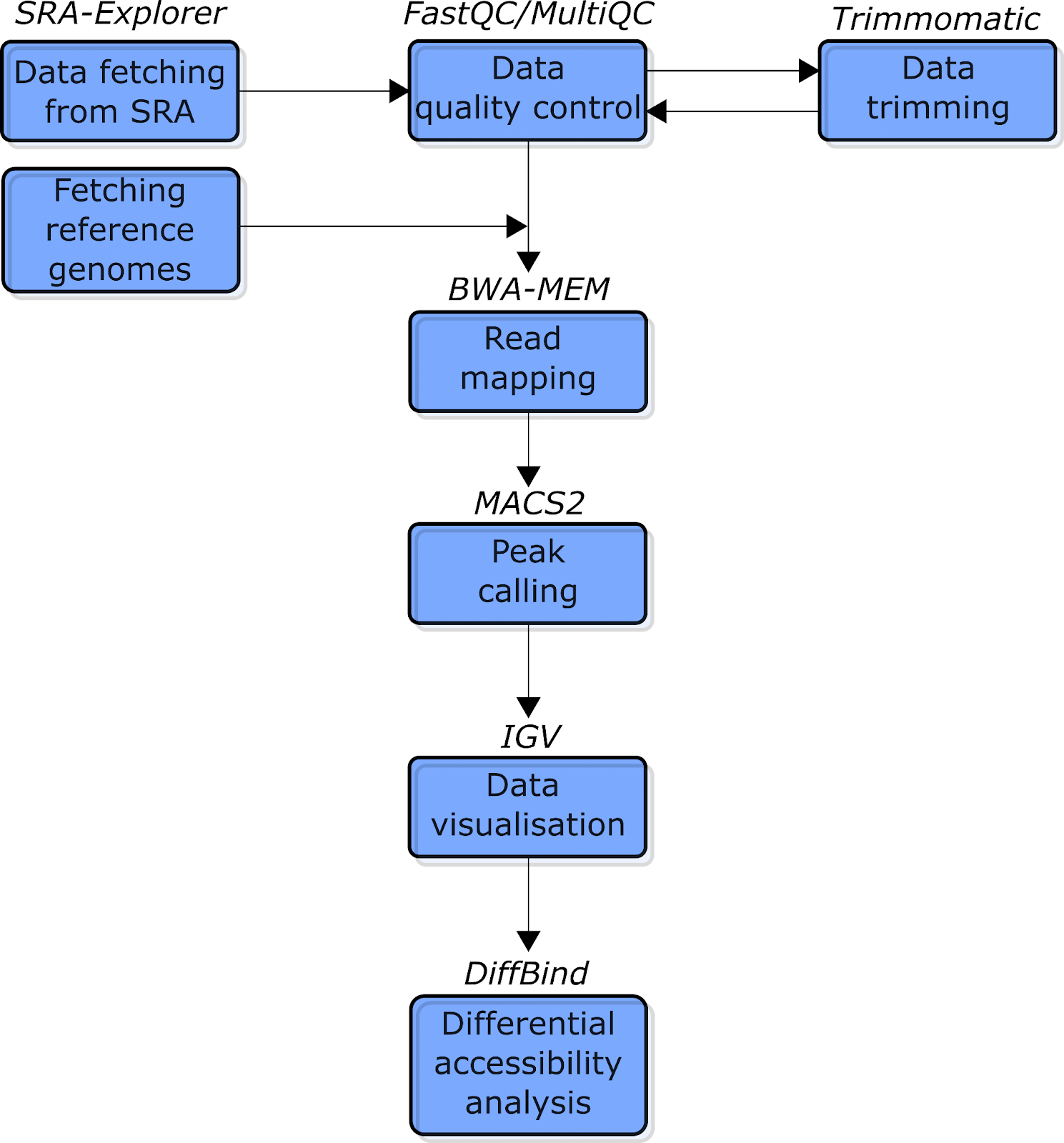
Fig. 2: The simplified schematic flowchart of the ATAC-seq data analysis pipeline covered in this tutorial. Blue boxes indicate the types of analysis. The text above the boxes indicates the software used for each analysis.
First, the data will be downloaded from Sequence Read Archive (SRA) using the online software SRA Explorer. After obtaining the data, we will run a quality control analysis using FastQC and MultiQC (Ewels et al. 2016) software to check and visualize the quality of the data, respectively. Next, we will use Trimmomatic (Bolger, Lohse, and Usadel 2014) software to remove the traces of Nextera adapter sequences that we introduced during the transposase integration process.
We now have clean data, and will use BWA (Li and Durbin 2009) software to map the reads against corresponding reference genomes. This will generate alignment files for further ATAC-seq peak calling, which we’ll do with the MACS2 (Zhang et al. 2008) package. Then the obtained data will be visualized with Integrative Genomic Viewer (Robinson et al. 2011). Finally, we will use the R DiffBind package (Ross-Innes et al. 2012) to run quality control and perform the differential chromatin accessibility analysis.
References
- Baek, Seungbyn, and Insuk Lee. 2020. “Single-Cell ATAC Sequencing Analysis: From Data Preprocessing to Hypothesis Generation.” Computational and Structural Biotechnology Journal 18 (June): 1429–39.
- Bolger, Anthony M., Marc Lohse, and Bjoern Usadel. 2014. “Trimmomatic: A Flexible Trimmer for Illumina Sequence Data.” Bioinformatics. https://doi.org/10.1093/bioinformatics/btu170.
- Buenrostro, Jason D., Beijing Wu, Howard Y. Chang, and William J. Greenleaf. 2015. “ATAC-Seq: A Method for Assaying Chromatin Accessibility Genome-Wide.” Current Protocols in Molecular Biology / Edited by Frederick M. Ausubel ... [et Al.] 109 (January): 21.29.1–21.29.9.
- Ewels, Philip, Måns Magnusson, Sverker Lundin, and Max Käller. 2016. “MultiQC: Summarize Analysis Results for Multiple Tools and Samples in a Single Report.” Bioinformatics 32 (19): 3047–48.
- Goodwin, Sara, John D. McPherson, and W. Richard McCombie. 2016. “Coming of Age: Ten Years of next-Generation Sequencing Technologies.” Nature Reviews. Genetics 17 (6): 333–51.
- Hovhannisyan, Hrant, Ester Saus, Ewa Ksiezopolska, Alex J. Hinks Roberts, Edward J. Louis, and Toni Gabaldón. 2020. “Integrative Omics Analysis Reveals a Limited Transcriptional Shock After Yeast Interspecies Hybridization.” Frontiers in Genetics 11 (May): 404.
- Johnson, Steven M., Frederick J. Tan, Heather L. McCullough, Daniel P. Riordan, and Andrew Z. Fire. 2006. “Flexibility and Constraint in the Nucleosome Core Landscape of Caenorhabditis Elegans Chromatin.” Genome Research 16 (12): 1505–16.
- Li, Heng, and Richard Durbin. 2009. “Fast and Accurate Short Read Alignment with Burrows-Wheeler Transform.” Bioinformatics 25 (14): 1754–60.
- Li, Heng, Bob Handsaker, Alec Wysoker, Tim Fennell, Jue Ruan, Nils Homer, Gabor Marth, Goncalo Abecasis, Richard Durbin, and 1000 Genome Project Data Processing Subgroup. 2009. “The Sequence Alignment/Map Format and SAMtools.” Bioinformatics 25 (16): 2078–79.
- Quinlan, Aaron R. 2014. “BEDTools: The Swiss‐Army Tool for Genome Feature Analysis.” Current Protocols in Bioinformatics. https://doi.org/10.1002/0471250953.bi1112s47.
- Robinson, James T., Helga Thorvaldsdóttir, Wendy Winckler, Mitchell Guttman, Eric S. Lander, Gad Getz, and Jill P. Mesirov. 2011. “Integrative Genomics Viewer.” Nature Biotechnology 29 (1): 24–26.
- Ross-Innes, Caryn S., Rory Stark, Andrew E. Teschendorff, Kelly A. Holmes, H. Raza Ali, Mark J. Dunning, Gordon D. Brown, et al. 2012. “Differential Oestrogen Receptor Binding Is Associated with Clinical Outcome in Breast Cancer.” Nature 481 (7381): 389–93.
- Song, Lingyun, and Gregory E. Crawford. 2010. “DNase-Seq: A High-Resolution Technique for Mapping Active Gene Regulatory Elements across the Genome from Mammalian Cells.” Cold Spring Harbor Protocols 2010 (2): db.prot5384.
- Yan, Feng, David R. Powell, David J. Curtis, and Nicholas C. Wong. 2020. “From Reads to Insight: A Hitchhiker’s Guide to ATAC-Seq Data Analysis.” Genome Biology. https://doi.org/10.1186/s13059-020-1929-3.
- Zhang, Yong, Tao Liu, Clifford A. Meyer, Jérôme Eeckhoute, David S. Johnson, Bradley E. Bernstein, Chad Nusbaum, et al. 2008. “Model-Based Analysis of ChIP-Seq (MACS).” Genome Biology 9 (9): R137.
Updated 5 months ago
