Read Mapping and Quantification
Runtime: See below for specific steps.
In this tutorial, our goal is to find genes that are differentially expressed between pathogenic and non-pathogenic forms of the human fungal pathogen C. parapsilosis. In order to assess differential expression, we first need to obtain “expression values” for genes of this yeast. In this section, we’ll show you how to calculate read counts for each gene (which are proportional to gene expression levels) using two different methods:
- The “classical” approach: Read mapping to a reference genome with subsequent calculation of mapped reads in each gene.
- The pseudo-mapping approach: Direct calculation of expression levels from the fastq files and reference transcripts.
There are advantages and disadvantages to each of these approaches. The main advantage of pseudo-mapping is that it’s extremely fast and requires very little RAM usage, while the classical approach is quite computationally demanding and can be relatively slow (depending on which software you use). Additionally, pseudo-mapping is just one step, while classical read-mapping involves two steps. (First read-mapping, then calculating the number of reads mapped to each gene.) Finally, read-mapping creates sam/bam files, which require a lot of hard drive space. Pseudo-mapping readily generates much smaller files with expression values.
On the other hand, a “classical” read mapping offers one important advantage over the pseudo-mapping approach: The large sam/bam read alignment files it creates allow us to perform many other valuable types of analysis on RNA-Seq data. That includes variant calling, novel transcript discovery, and calculation of species proportions when several organisms are sequenced as one sample (for example in case of host-microbe interaction studies, metatranscriptomics studies, etc.). In contrast, pseudo-mapping has far more limited applications, and is mainly used to assess gene expression levels.
In a normal RNA-Seq analysis, your choice of read-mapping method will depend on the specific research question you’re investigating. In this tutorial, we’ll show you how to perform both of these approaches.
Reference genome fetching
For both read-mapping methods, we will need a reference genome and genome annotations. Our first step is to obtain that data from a special database for Candida species called Candida Genome Database. Go go to the ref_gen directory and download both files with the following commands:
wget http://www.candidagenome.org/download/sequence/C_parapsilosis_CDC317/current/C_parapsilosis_CDC317_current_chromosomes.fasta.gz
wget http://www.candidagenome.org/download/gff/C_parapsilosis_CDC317/C_parapsilosis_CDC317_current_features.gff
gunzip C_parapsilosis_CDC317_current_chromosomes.fasta.gz
In this code, the wget commands will download the reference genome and genome annotation in gff format for C. parapsilosis. The gunzip command will uncompress the genome file. With these two files, we can perform both read mapping and pseudo-mapping.
Read mapping and counting using STAR software
First, we will perform read mapping and read calculation using STAR – a popular, versatile software package for RNA-Seq read-mapping. STAR is very fast, offers a wide variety of options and analyses, and comes with excellent user support. Another important advantage of STAR is that it can calculate the number of reads mapped to each gene during the mapping process, so we won’t need to use any additional software. For our analysis of yeast data, STAR will need just 2-3 GB of RAM.
To use STAR, let's first install it in our rnaseq environment. Run this command:
conda install star --channel conda-forge --channel bioconda --channel defaults --strict-channel-priorityTo begin read mapping, we first need to index the reference genome:
Index the reference genome:
Run time ~10 seconds on workstation, 20 seconds on mac
To index the genome, first run the following command:
STAR --runThreadN 2 --runMode genomeGenerate --genomeDir cpar --genomeFastaFiles C_parapsilosis_CDC317_current_chromosomes.fasta --genomeSAindexNbases 10Before proceeding, let’s explore what this command is doing:
--runThreadN 2 tells STAR to use 2 cores
--runMode genomeGenerate tells STAR to perform genome indexing
--genomeFastaFiles sets the genome to be indexed (C_parapsilosis_CDC317_current_chromosomes.fasta)
--genomeDir cpar tells STAR to write the index to the cpar directory.
--genomeSAindexNbases is specific to our genome. We are setting the value to 10 (vs. the default value of 14) because the size of the C. parapsilosis genome is small.
See the STAR manual for more details on these parameters.
Convert the file format of genome annotations
The final step before we can perform read mapping is to convert the original genome annotations (which are in gff format) to gtf format. This is necessary because gtf is the preferred format for STAR to count reads for downstream differential gene expression analysis. For this conversion, we'll use the gffread tool (Pertea and Pertea 2020).
First, install gffread in the environment:
conda install gffread --channel conda-forge --channel bioconda --channel defaults --strict-channel-priorityNow run gffread with this command:
gffread C_parapsilosis_CDC317_current_features.gff -T -o C_parapsilosis_CDC317_current_features.gtfRead mapping
Runtime: ~20 min on the Workstation, ~1 hour on the Mac
Now that we have indexed the reference genome and converted the original annotations to gtf format, we can proceed with the actual read mapping. First, go to the mapping directory with this command:
cd ../mapping/To run the read mapping for all samples, we will use the following script:
while read f; do
echo "STAR --runThreadN 2 --genomeDir ../ref_gen/cpar/ --sjdbGTFfile ../ref_gen/C_parapsilosis_CDC317_current_features.gtf --readFilesIn ../raw_data/trimming/${f}_tr_1P.fastq.gz ../raw_data/trimming/${f}_tr_2P.fastq.gz --readFilesCommand zcat --outFileNamePrefix ${f}_ --outSAMtype BAM SortedByCoordinate --limitBAMsortRAM 3000000000 --quantMode GeneCounts”
done<../raw_data/sample_ids.txt
This simple script will iterate over the file names we have written in the raw_data/sample_ids.txt file and print the STAR command for each file. Let’s explore this script in greater detail:
--runThreadN 2 tells STAR to use 2 CPU cores (change this number if you have more/fewer cores)
--genomeDir navigates STAR to the reference genome index
--sjdbGTFfile navigates to the gtf file
--readFilesIn specifies the trimmed input files for each sample
--readFilesCommand zcat is necessary to read the fastq files in a compressed format (Note: if you are using a Mac computer, change “zcat” to “gzcat”.)
--outFileNamePrefix ${f}_ specifies the prefix of the output files
--outSAMtype BAM SortedByCoordinate tells STAR to generate sorted bam files
--limitBAMsortRAM 3000000000 directs STAR to use a maximum 3 GB of RAM for bam file sorting (which is enough in our case)
--quantMode GeneCounts tells STAR to perform read calculation for each gene, generating the values that we need for differential expression analysis.
Now run this command:
bash mapping.sh > star_commands.txtThis will output all the above-mentioned commands to a file called star_commands.txt. As in our trimming step, this file can be either run as a bash command or submitted as an array job in computing clusters. Here we will use the bash command:
bash star_commands.txt Note for Mac users
If STAR 2.7.10a throws a “Segmentation fault” error when the mapping step starts, please install an older version of STAR.
Upon finishing the read mapping for each sample, STAR produces several output files. Their names will begin with the value we set via the --outFileNamePrefix option (i.e. with the corresponding sample name). Our main output files will be the following:
- Aligned.sortedByCoord.out.bam – a sorted read alignment file in bam format
- Log.final.out – a final concise log file of STAR mapping
- ReadsPerGene.out.tab – a file containing the read count data which will be used for differential gene expression analysis
Checking success of read mapping
To ensure our read mapping was successful, let's inspect several parameters in the Log.final.out files. Open the file SRR1278968_Log.final.out, and let's review these three parameters:
- Uniquely mapped reads %
- % of reads mapped to multiple loci
- % of reads unmapped: too short
Uniquely mapped reads % tells us what percentage of total reads were mapped uniquely to the reference genome. The higher this number is, the better. Values between 85% and 95% are considered a good mapping rate. In our case, that number is 96.80%, which is quite high.
% of reads mapped to multiple loci indicates the percentage of reads that are mapped to more than one genomic position. These are called multi-mapped reads, and it’s difficult to know their true place of origin. The multimapping rate is typically high for samples originating from genomes with highly repetitive regions, preventing the software from mapping the reads uniquely to those regions. In our case, the multimapping rate is 2.21%, which is low.
% of reads unmapped: too short indicates the percentage of reads that did not map to the reference because the alignment of that read to the genome was too short. Obviously, the lower this number is, the better. For our sample, the unmapped reads constitute only 0.98%.
So far, we have only reviewed one of many log files. To simplify this process, we can aggregate the statistics from many log files using MultiQC. In the mapping folder, run this command:
multiqc .When the analysis is finished, open the file multiqc_report.html in your browser. You should see an image like the one below (Fig. 7), which nicely illustrates our mapping statistics in a single plot:
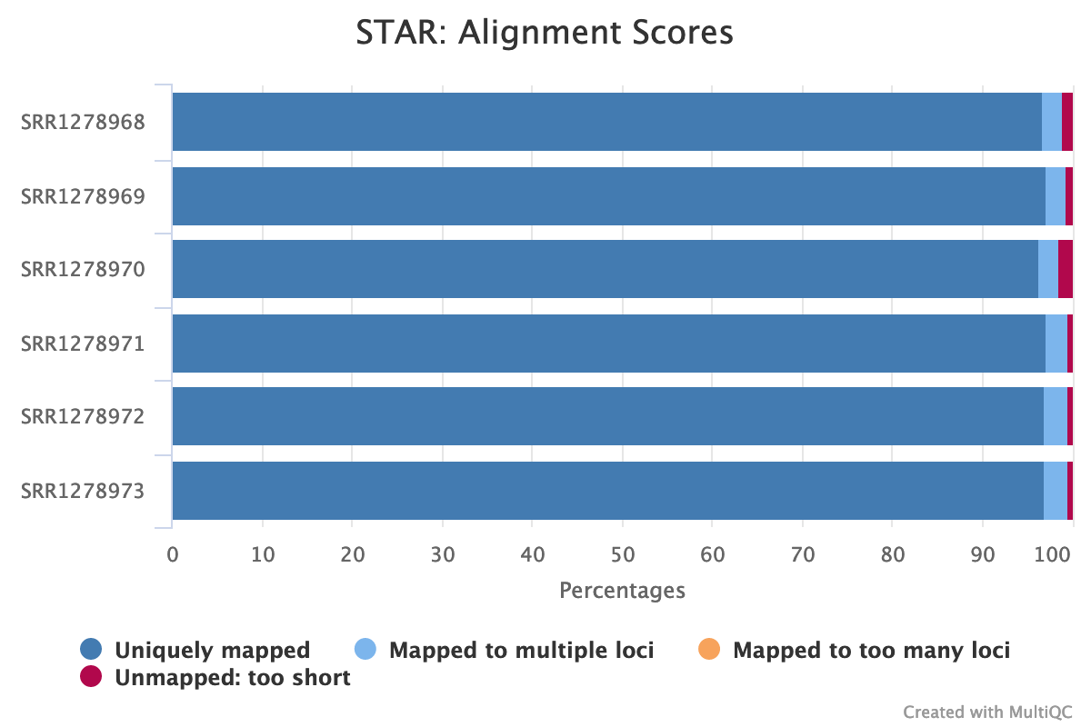
Fig. 7: An aggregated plot of STAR mapping statistics for all analyzed samples.
As we discussed above, STAR also generates ReadsPerGene.out.tab files, which contain read counts of genes (i.e. how many reads were mapped to each gene) in C. parapsilosis. Let’s review one example – the file SRR1278968_ReadsPerGene.out.tab. This file has four columns which correspond to different strandedness options:
- Column 1 – gene name
- Column 2 – counts for unstranded RNA-seq
- Column 3 – counts for forward-stranded data
- Column 4 – counts for the reverse-stranded data
We already know that our data is stranded, per the original paper by Holland et al., 2014. And in the MultiQC plot called “Gene Counts” (Fig. 8, below) we can clearly see that most reads are assigned to genes in reverse-stranded configuration:
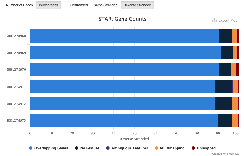
Fig. 8: Reads counts of all samples depending on strandedness configuration.
This means that our RNA-Seq data is reverse-stranded. Thus, we will need to use the data in column 4 for differential gene expression analysis. More details about RNA-Seq strandedness can be found here and here.
We have now performed read mapping for all RNA-Seq samples of C. parapsilosis using STAR mapper. The software has additionally calculated the number of reads mapping to each gene. This data will be used later to perform differential gene expression analysis.
Visualization of RNA-Seq bam files
Runtime: Depends on how long you spend investigating the data.
In this section, we will visualize the bam files we obtained during read mapping to make our analysis more intuitive and clear. We will use Integrative Genomics Viewer (Robinson et al. 2011) (IGV), which is a powerful and versatile java application for visualizing genomics data. But before our bam files can be visualized, they must first be sorted and indexed. They have already been sorted via STAR mapper, which we used for read mapping. To index them, we will use the program samtools (Li et al. 2009).
First, install samtools in the rnaseq environment using this command:
conda install samtools --channel conda-forge --channel bioconda --channel defaults --strict-channel-priority Now let’s index one of the bam files that we have generated in the previous step. Run the following command:
samtools index SRR1278973_Aligned.sortedByCoord.out.bamNext, install and launch IGV with these commands:
conda install -c bioconda igv
igv
This will open a graphical user interface for the program. Go to Genome > Load Genomes from File > select the genome fasta file of C. parapsilosis. The chromosomes of the yeast will appear at the top of IGV. Now go to File > Load from file > select the gff annotation file of C. parapsilosis. The genome annotations will appear underneath the chromosome, showing genes and other annotated elements of the genome. We can right-click on the annotations track, and select the “Expanded” option to see all genomic features more clearly. Next, go to File > Load from file > select the indexed bam file SRR1278973_Aligned.sortedByCoord.out.bam.
When this file is selected, IGV will create two tracks – one with a coverage line plot (at the top), and a second, larger track visualizing all mapped reads. To see both of these plots, select one chromosome from the dropdown menu, then zoom in using the + sign at the top-right corner. After zooming in sufficiently, the coverage plot and the reads will appear. They should look like this:
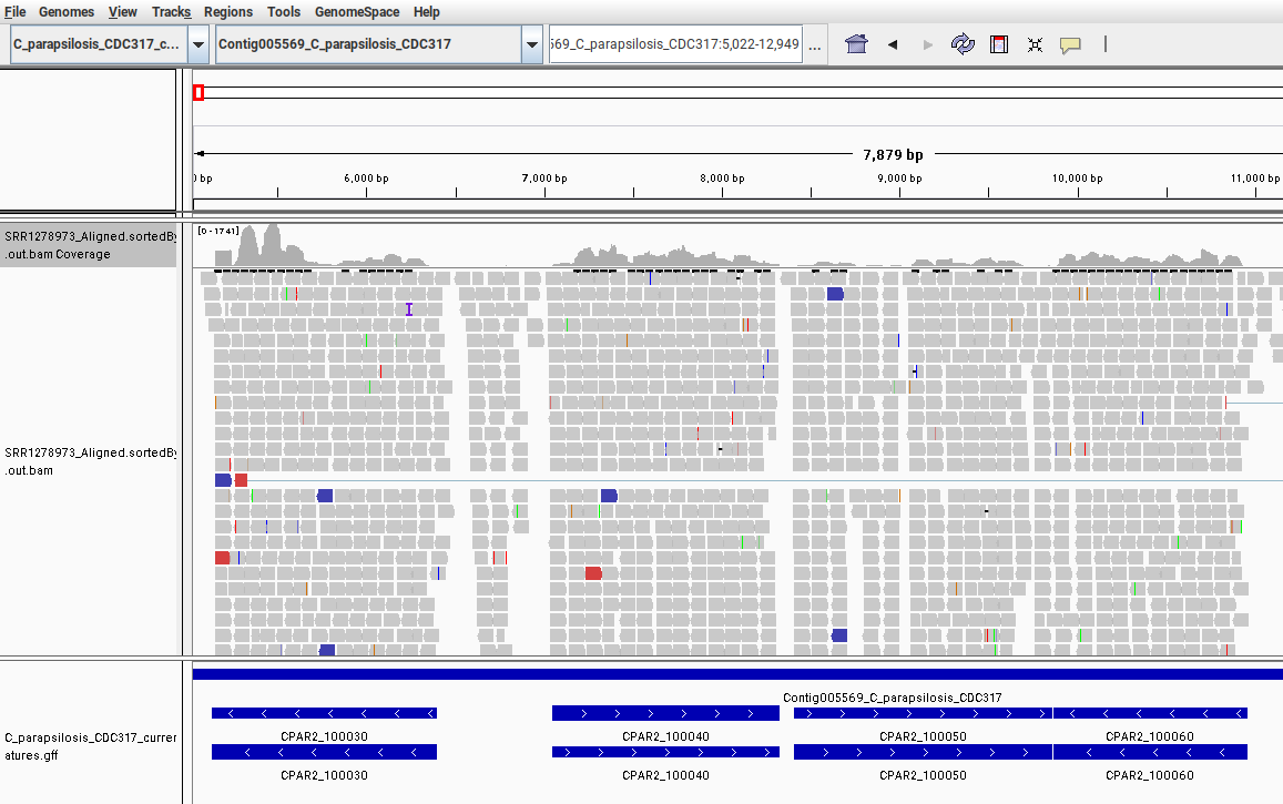
Fig. 9: Screenshot from IGV showing the mapped RNA-Seq data to the C. parapsilosis reference genome. Only a small region in the beginning of the chromosome “Contig005569” is shown.
In this image, we can see that different genes have different coverages. This means that each gene has a different number of reads mapped to it, reflecting its expression levels. In our read-counting section, we counted the number of mapped reads that fall within the range of each gene. We have now visualized these relationships with IGV.
Get to know Integrative Genome Viewer (IGV)
IGV is very powerful, flexible software that can visualize and analyze many other features of mapped reads. We highly recommend spending more time with it to explore its many functions!
Read quantification using Salmon software
Runtime: See below for indexing and pseudo-mapping steps.
In this section, we will explore an alternative approach to calculating read counts in each gene from our RNA-Seq samples. We will use Salmon software, which performs a so-called pseudo-mapping (or pseudo-alignment) analysis to directly quantify the read counts and expression levels of genes from fastq files and reference transcripts. Salmon and similar software such as kallisto (Bray et al. 2016), are extremely fast, require very little RAM, and do not produce the “classical” sam/bam alignment files, which require a lot of storage space.
To perform this analysis, we will need to complete three steps:
- Obtain a fasta file of genes/transcripts of C. parapsilosis
- Index that fasta file
- Perform pseudo-mapping
We’ll use gffread to perform the first step, and Salmon to perform the second and third steps.
First let's install both software packages. We recommend installing them in a new, separate conda environment. The following command both creates a new salmon_env environment and installs Salmon and gffread software to it:
conda create -n salmon_env salmon gffread  --channel conda-forge --channel bioconda  --channel defaults --strict-channel-priority
conda activate salmon_env
Obtain a fasta file of genes/transcripts ofC. parapsilosis
Next, let's obtain the fasta file with gene sequences for C. parapsilosis. We’ll use gffread, which extracts the gene sequences from the reference genome of C. parapsilosis based on the information of the gff file. In the ref_gen directory, run this command:
gffread -w transcripts.fasta -W -F -g C_parapsilosis_CDC317_current_chromosomes.fasta C_parapsilosis_CDC317_current_features.gffThis command creates the file transcripts.fasta, which contains the sequences of C. parapsilosis genes (based on exon information in gff files)
Now let’s create two new directories in our initial folder and go to the first one:
mkdir -p salmon/ref_gen salmon/mapping
cd salmon/ref_gen/
Index the fasta file with Salmon
Runtime: 5 seconds on the Workstation, 30 seconds on the Mac
Next, we will create an index of the transcripts.fasta file called cpar_index, to which we then will perform the pseudo-mapping. Run the following commands to perform the indexing:
salmon index -t ../../ref_gen/transcripts.fasta -i cpar_indexPerform pseudo-mapping
Runtime: 4 min on the Workstation, 15 minutes on the Mac
Once the indexing is finished, we can perform the pseudo-mapping. First, switch to the salmon/mapping directory:
cd ../mapping/Now run the following script called salmon_mapping.sh:
while read f;do
echo "salmon quant -i ../ref_gen/cpar_index/ -l A" \
"-1 ../../raw_data/trimming/${f}_tr_1P.fastq.gz" \
"-2 ../../raw_data/trimming/${f}_tr_2P.fastq.gz" \
"-p 2 --validateMappings -o quants/${f}_quant"
done<../../raw_data/sample_ids.txt
As in our previous trimming and read mapping steps, this script iterates over the sample names in the sample_ids.txt file, and for each sample prints out a salmon command for pseudo-mapping. Let’s review this command in more detail:
-i directs Salmon to the cpar_index
-l A tells Salmon to automatically detect strandedness of data
-1 and -2 supply the reads to Salmon
-p 2 tells Salmon to use 2 cores
--validateMappings increases sensitivity of Salmon
-o specifies the name of the output folders.
To generate these Salmon commands, run this command:
bash salmon_mapping.sh > salmon_commands.txt
Finally, use this command to run Salmon:
bash salmon_commands.txtUpon completing this task, Salmon will produce several output files. The file salmon_quant.log will contain information about mapping rates. To aggregate the result of all samples, we can use MultiQC. Run MultiQC with this command:
multiqc .Now open the generated report in your browser. The general statistics and mapping rates should look like this:
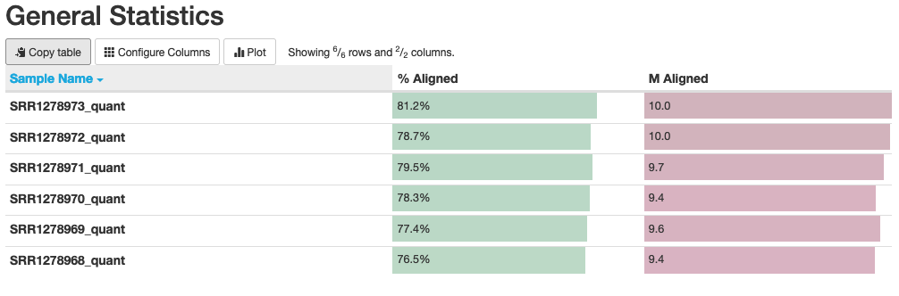
Fig. 10: General statistics and mapping rates of Salmon runs.
In this plot, we can see that our “% Aligned” data averages around 78%, which is lower than the number we found when read mapping via STAR. This is somewhat expected because Salmon “aligns” the reads only to known genes/transcripts that we supply to it, while STAR maps reads to the entire genome and can capture data originating from non-annotated genes/transcripts.
The main output file of Salmon, which contains the gene expression data, is called quant.sf. Let's open the file quants/SRR1278968_quant/quant.sf. This file has 5 columns:
- Name - gene/transcript name
- Length - gene/transcript length
- EffectiveLength - gene/transcript effective length (see here for details)
- TPM - Transcripts Per Million (TPM) expression levels (see more details about this in the following sections)
- NumReads - an estimated number of reads “mapped” to genes/transcripts
The data in our final column – NumReads – can be used for differential gene expression analysis.
To summarize, we have just performed a fast, lightweight read counting with pseudo-mapping using Salmon software. We can now move on to differential gene expression analysis.
Works Cited
- Bray, N. L., H. Pimentel, P. Melsted, and L. Pachter. 2016. “Near-Optimal Probabilistic RNA-Seq Quantification.” Nature Biotechnology 34 (5). https://doi.org/10.1038/nbt.3519.
- Holland, L. M., M. S. Schröder, S. A. Turner, H. Taff, D. Andes, Z. Grózer, A. Gácser, et al. 2014. “Comparative Phenotypic Analysis of the Major Fungal Pathogens Candida Parapsilosis and Candida Albicans.” PLoS Pathogens 10 (9). https://doi.org/10.1371/journal.ppat.1004365.
- Li, H., B. Handsaker, A. Wysoker, T. Fennell, J. Ruan, N. Homer, G. Marth, G. Abecasis, and R. Durbin. 2009. “The Sequence Alignment/Map Format and SAMtools.” Bioinformatics 25 (16). https://doi.org/10.1093/bioinformatics/btp352.
- Pertea, G., and M. Pertea. 2020. “GFF Utilities: GffRead and GffCompare.” F1000Research 9 (April). https://doi.org/10.12688/f1000research.23297.2.
- Robinson, James T., Helga Thorvaldsdóttir, Wendy Winckler, Mitchell Guttman, Eric S. Lander, Gad Getz, and Jill P. Mesirov. 2011. “Integrative Genomics Viewer.” Nature Biotechnology 29 (1): 24.
Updated 4 months ago